Homework 05
Alfven current
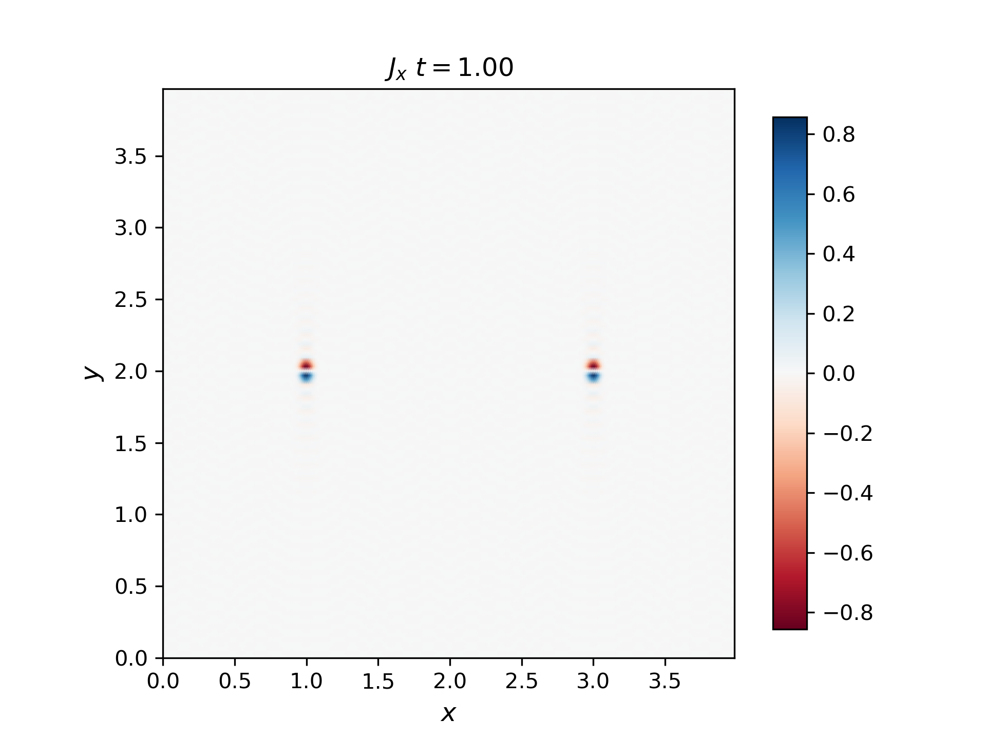
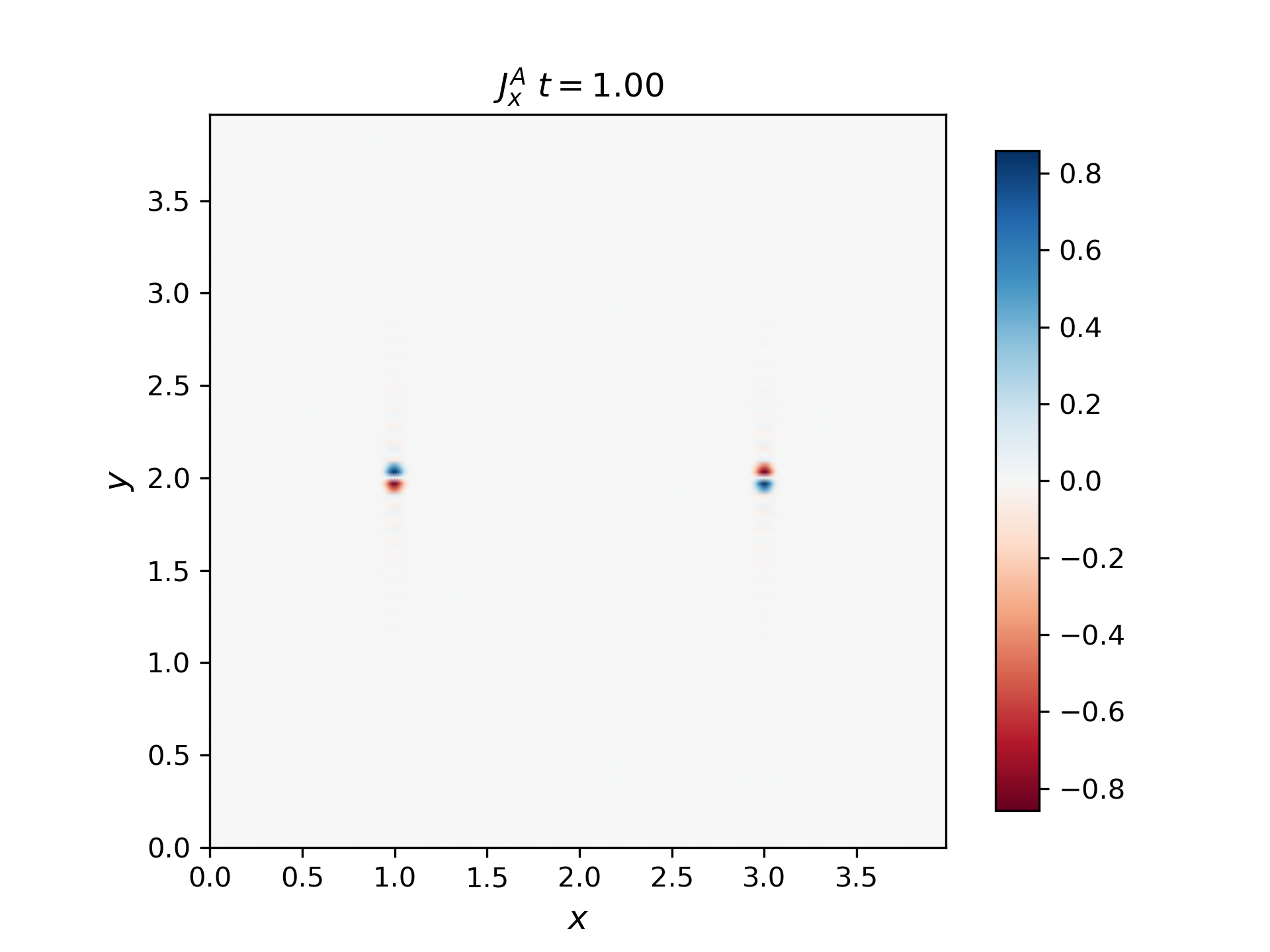
Compute the parallel current from a bipolar Alfvén wavepacket. In the simulation lecture it was shown that a unipolar pulse (magnetic bomb, Bz unipolar gaussian) creates a field aligned current. The direction of that current was computed from curlB (left panel in the 2D result) and (in simulation coordinates) from \(J_x=[±1/(μ_0 C_a)] dE_y/dy\) (right panel in the 2D result).
Unipolar Alfvén wavepacket
Multiply the RHS image by the sign corresponding to the propagation direction, we get the LHS image.
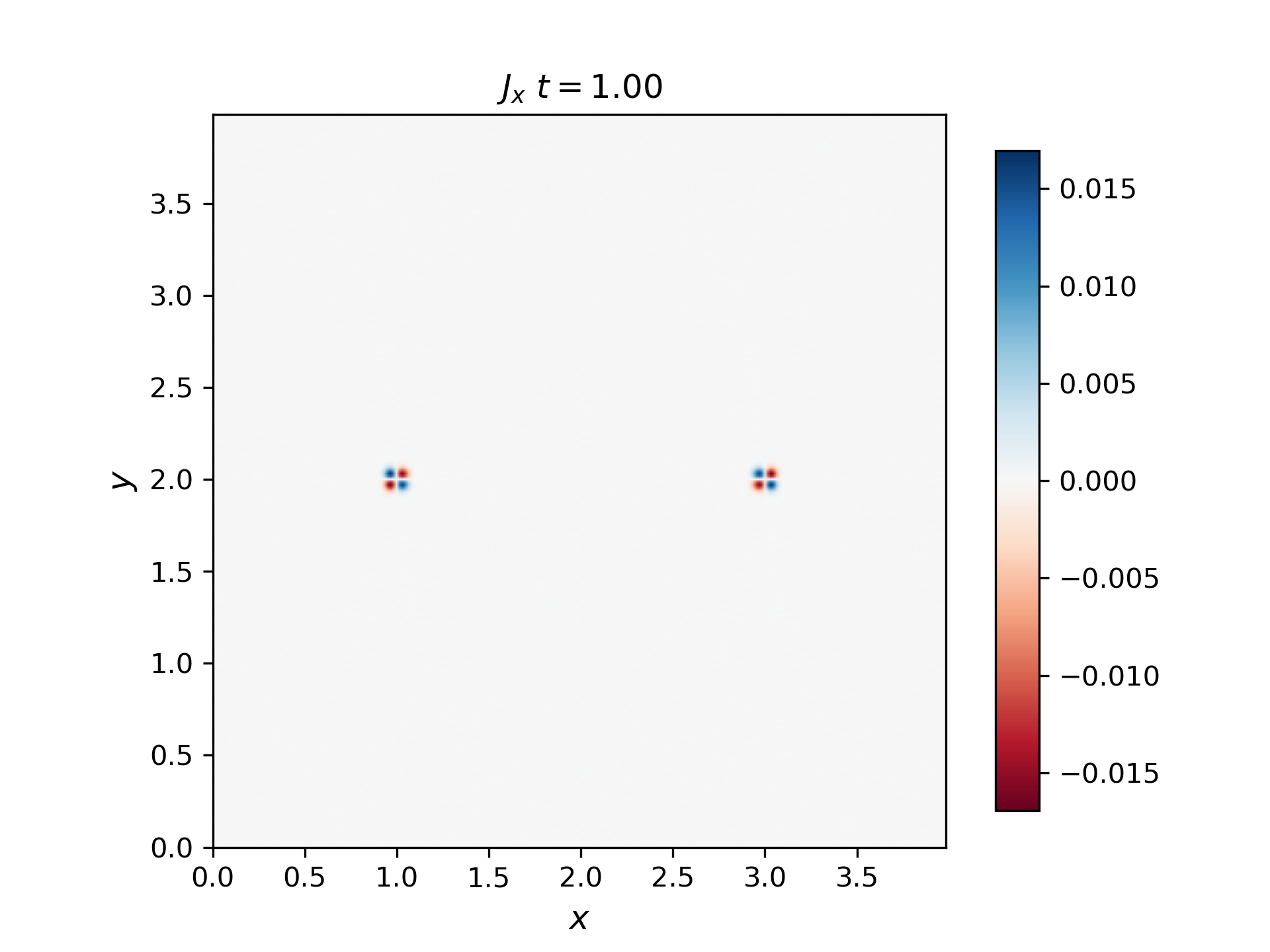
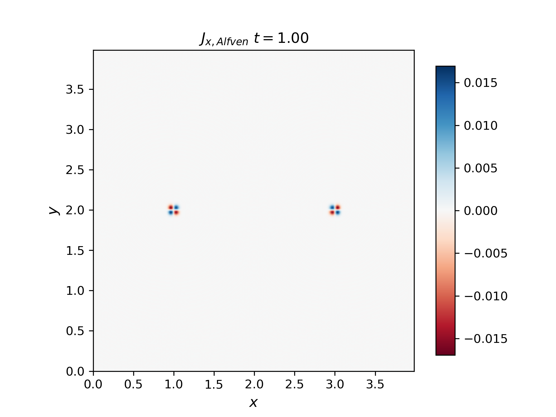
Bipolar Alfvén wavepacket
To create a bipolar pulse in dBz and let it evolve on both sides. The init input is as follows:
case(6)
    !2D gaussian perturbation in Bz modulated by a odd function of x
    do iz = izmin,izmax
        do iy = iymin,iymax
            do ix = ixmin,ixmax
                uu(ix,iy,iz,7) = uu(ix,iy,iz,7) + db0 * (xgrid(ix) - 0.5*Lx) * &
                exp( -( (xgrid(ix)-0.5*Lx)/(0.01*Lx) )**2 - ((ygrid(iy)-0.5*Ly)/(0.01*Ly))**2)
            enddo
        enddo
    enddo
The basic idea is to change the amplitude modulation part from a constant to a odd function like (xgrid(ix) - 0.5*Lx) (sin would also work).
The figures below show the current density in the x direction for the bipolar Alfvén wavepacket.
The notebooks to reproduce the results are available here with initial input here.
Hydrodynamic shock
Show that the entropy across a hydrodynamic shock increases: (i) First, prove equation III.80 in Siscoe (you can use the jumps in p and \(ρ\) previously derived). (ii) Next, take the derivative of the entropy ratio as function of Mach number and show it is positive. Thus explain that starting from M1=1 and moving upwards all M1 values have positive entropy ratios. (iii) Plot the entropy ratio as function of M1 for a range of adiabatic indices. (iv) Under what conditions does the entropy not increase? [Ans. \(γ=1\)] When might such conditions occur in space plasmas and why? [Ans. parallel shocks]
Given the jump conditions of pressure and density:
\[ \rho _2\to \frac{(γ +1)}{γ +\frac{2}{M_1^2}-1} \rho _1 \] \[ p_2\to \frac{\left(2 γ M_1^2-(γ -1)\right)}{γ +1} p_1 \]
And as the entropy is defined as \(\alpha_i\text{:=} p_i / \rho _i^{γ}\)
assums = { Subscript[ρ, 1] > 0, γ > 0, Subscript[M, 1] > 0};
ratio = Simplify[α[2]/α[1] /. rules, assums]
gives us
\[ α[2]/α[1] = (γ +1)^{-γ -1} \left(γ +\frac{2}{M_1^2}-1\right)^{γ } \left(-γ +2 γ M_1^2+1\right) = \left(\frac{1}{γ+1}\right)^{γ+1}\left[2 γ M_1^2-(γ-1)\right]\left(γ-1+\frac{2}{M_1^2}\right)^γ \]
Taking the derivative of the entropy ratio with respect to \(M_1\):
dRatio = D[ratio, M1];
dRatio = Simplify[dRatio, assums];
dRatio /. formatRules
gives us
\[ \frac{d}{d M_1} \left(\frac{α_2}{α_1}\right) = 4 (γ -1) γ (γ +1)^{-γ -1} \left(M_1^2-1\right)^2 M_1^{-2 γ -1} \left((γ -1) M_1^2+2\right)^{γ -1} \]
The derivative is positive for all \(M_1>0\) values as long as \(γ>1\). And when \(M_1=1\), the ratio is equal to 1.
The plot of the entropy ratio as a function of \(M_1\) for a range of adiabatic indices is shown below.
γs = {1, 4/3, 5/3, 2};
LogLogPlot[
 Evaluate[ratio /. γ -> γs], {M1, 1, 100},
 PlotLegends -> γs
 ]
And we can see that when \(γ=1\), the entropy ratio is constant and equal to 1. As \(p = α_1 ρ^γ = n k T\), this corresponds to the case where the temperature is constant across the shock. Isothermal behavior is due to fast, field-aligned escaping electrons and this is more likely to occur in parallel shocks.
The mathematica notebook for this question and the following question is available here.
Perpendicular Shock
- Show Eq. III.90 following Siscoe notes. Follow same procedure as in III.73 to factor the known solution and derive the quadratic coefficients. Write (X-1)(X^2 + A_1 X + A_0)=0 where X = (U2/U1) and solve for A0 and A1 given the coefficients of the cubic. For extra testing of cubic, make sure that X=1 is indeed a valid solution. As another test of your cubic equation (you can do that always during the derivation): Set \(A_1 → ∞\) and validate it becomes a quadratic that is identical to III.71 (with M1 defined same as S1).
The continuity relations for the perpendicular shock can be written as \[ \begin{aligned} & [[\rho U]]=0 \\ & \left[\left[\rho U^2+p+\frac{B^2}{2 \mu_0}\right]\right]=0 \\ & {\left[\left[\left(\frac{1}{2} \rho U^2+\frac{\gamma}{\gamma-1} \rho+\frac{B^2}{\mu_0}\right) U\right]\right]=0} \\ & {[[U B]]=0} \end{aligned} \]
Normalizing the magnetic pressure by the ram pressure and the thermal pressure by the ram pressure
\[ B_1^2\to \frac{\rho _1 U_1^2}{A^2} \] \[ p_1\to \frac{\rho _1 U_1^2}{\gamma S^2} \]
And Elimitating \(B_2\), \(\rho_2\) and \(p_2\) from the equations
massEq := \[Rho]1 U1 == \[Rho]2 U2
momEq := \[Rho]1 U1^2 + p1 + B1^2/2 == \[Rho]2 U2^2 + p2 + B2^2/2
energyEq := (1/2 \[Rho]1 U1^2 + f p1 + B1^2) U1 == (1/2 \[Rho]2 U2^2 +
      f p2 + B2^2) U2
FaradayEq := B1 U1 == B2 U2
eqs = {massEq, momEq, energyEq, FaradayEq};

Simplify[
 Eliminate[eqs, {B2, \[Rho]2, p2}] /. rules, {Subscript[U, 1] > 0,
  Subscript[\[Rho], 1] > 0}]
We get the following equation
\[ \frac{(r-1) \left(A^2 r \left(S^2 (-\gamma +\gamma r+r+1)-2\right)+S^2 (\gamma +\gamma (-r)-2)\right)}{A (\gamma -1) S}=0 \]
where \(r = U_2/U_1\).
Clearly, \(r=1\) is a solution. We can collect the rest equation to get the quadratic equation in \(r\)
Collect[S^2 (-2 + \[Gamma] - r \[Gamma]) + A^2 r (-2 + S^2 (1 + r - \[Gamma] + r \[Gamma])) == 0, r]we get
\[ r^2 \left(A^2 \gamma S^2+A^2 S^2\right)+r \left(-A^2 \gamma S^2+A^2 S^2-2 A^2-\gamma S^2\right)+\gamma S^2-2 S^2=0 \]
This is exactly the same as Eq. III.90 in Siscoe notes.
- Solve the quadratic to find the two solutions for U2. Show that one is non-physical, and identify the remaining, physical one.
assums = {A > 0 , S > 0, \[Gamma] > 1};
Solve[eqR, {r}, Reals, Assumptions -> assums] // Simplify
Solve the quadratic equation, we get
\[ \left\{\left\{r\to \frac{A^2 \left((\gamma -1) S^2+2\right)-\sqrt{A^4 \left((\gamma -1) S^2+2\right)^2+A^2 \left(\left(-2 \gamma ^2+2 \gamma +8\right) S^4+4 \gamma S^2\right)+\gamma ^2 S^4}+\gamma S^2}{2 A^2 (\gamma +1) S^2}\right\},\left\{r\to \frac{A^2 \left((\gamma -1) S^2+2\right)+\sqrt{A^4 \left((\gamma -1) S^2+2\right)^2+A^2 \left(\left(-2 \gamma ^2+2 \gamma +8\right) S^4+4 \gamma S^2\right)+\gamma ^2 S^4}+\gamma S^2}{2 A^2 (\gamma +1) S^2}\right\}\right\} \]
The first solution is non-physical as it is negative. The physical solution is
\[ r_1\text{:=}\frac{A^2 \left((\gamma -1) S^2+2\right)+\sqrt{A^4 \left((\gamma -1) S^2+2\right)^2+A^2 \left(\left(-2 \gamma ^2+2 \gamma +8\right) S^4+4 \gamma S^2\right)+\gamma ^2 S^4}+\gamma S^2}{2 A^2 (\gamma +1) S^2} \]
In the limit of \(A\to\infty\)
Subscript[r, 1] :=
 1/(2 A^2 S^2 (1 + \[Gamma])) (A^2 (2 + S^2 (-1 + \[Gamma])) +
    S^2 \[Gamma] + \[Sqrt](A^4 (2 + S^2 (-1 + \[Gamma]))^2 +
       S^4 \[Gamma]^2 +
       A^2 (4 S^2 \[Gamma] + S^4 (8 + 2 \[Gamma] - 2 \[Gamma]^2))))
Simplify[Limit[Subscript[r, 1], {A -> \[Infinity]}], assums]
we can see that the solution becomes
\[ \frac{(\gamma -1) S^2+2}{(\gamma +1) S^2} \]
which is the same as Eq. III.71 in Siscoe notes for hydrodynamic shocks.
- Plot the solution as function of A1 and M1 (color, contour or surface plot OK). Show that the limits for \(A_1→∞\) and \(M_1→∞\) are as expected.
In the limit of \(A_1→∞\) and \(M_1→∞\), the solution approaches \(\frac{\gamma -1}{\gamma +1}\). For \(γ=5/3\), the solution approaches 0.25, which is expected. The contour plot of the solution is shown below.
Block[{\[Gamma] = 5/3, p1, p2},
 p1 = ContourPlot[r1, {A, 0, 100}, {S, 0, 100},
   PlotLegends -> Automatic];
 p2 = ContourPlot[r1, {A, 0, 10}, {S, 0, 10},
   PlotLegends -> Automatic];
 Export["figures/shock_U2.svg", p1];
 Export["figures/shock_U2_zoom.svg", p2];
 {p1, p2}
 ]
