Code
using Pkg
Pkg.add([
    "YAML",
    "DataFrames",
    "Gadfly",
    "Unitful",
])

using YAML
using DataFrames
using Gadfly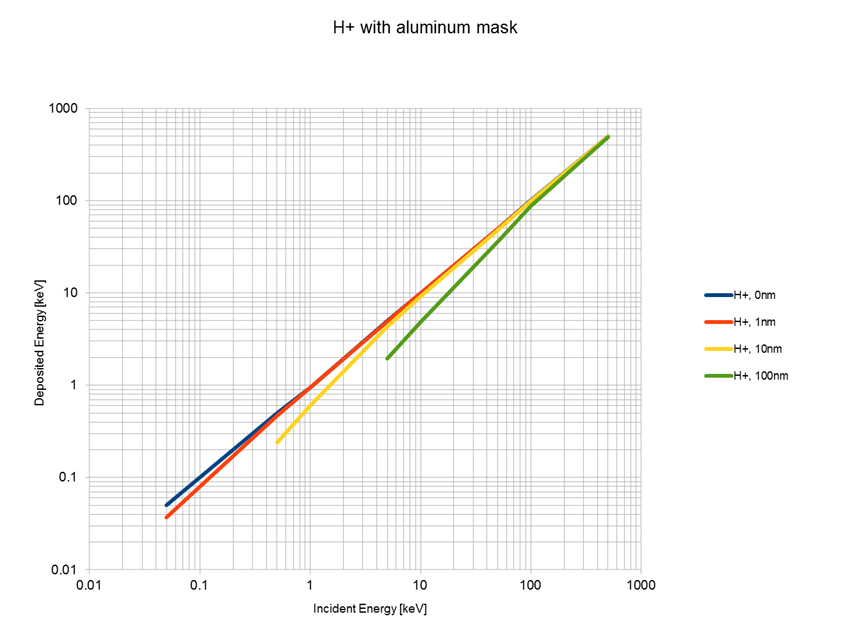
using UnitfulPlot the energy recorded (past the Al) versus the incident energy, for beams of various energies, and for different thickness (10nm, 100nm, …). Use H+, He+, O+. Use SPENVIS or GEANT-4 for your modeling.
The energy loss of particles depends on the nature of particles (mass, charge, etc), the incident energy, and the thickness of the Al layer.
For the two-layer detector, where the first layer is Al and the second layer is Silicon, the thickness of the Al layer varies from 0 nm to 100 nm with the thickness of the Si layer fixed to 2 mm.
As shown in Figure 1, heavier ions like O+ deposits more energy in the Al layer than lighter ions like He+ and H+, leading to a smaller energy recorded by the Si layer.
And for O+ with low incoming energy below a certain energy threshold \(E\), the recorded deposited energy in Si layer will drop to zero. This threshold energy \(E\) depends on the thickness of the Al layer \(d\). The thicker the Al layer, the higher the threshold energy.
\[E=E(d)\]
More generally, the threshold energy \(E\) also depends the incident particle \(s\).
\[E=E(d,s)\]
using Pkg
Pkg.add([
"YAML",
"DataFrames",
"Gadfly",
"Unitful",
])
using YAML
using DataFrames
using Gadfly
using Unitfulfunction parse_result_line(line)
values = split(line, ',')
Layer = parse(Int, values[1])
Thickness = parse(Float64, values[2]) # Assuming thickness in cm
Density = parse(Float64, values[3]) # Assuming density in g/cm3
Dose = parse(Float64, values[4]) # Assuming dose in keV
Error = try
parse(Float64, values[5])
catch _
NaN
end # Handle '-nan' and other errors
return (Layer, Thickness, Density, Dose, Error)
end
function convert_data(yaml_data)
# Iterate through the data and convert each field
for entry in yaml_data
entry["layer.Al.thickness"] = parse(Float64, replace(entry["layer.Al.thickness"], " um" => "")) * 1000 * u"nm"
entry["source"]["energy"] = parse(Float64, replace(entry["source"]["energy"], " MeV" => "")) * 1000
entry["result"] = [parse_result_line(line) for line in split(entry["result"], '\n') if line != ""]
end
df = DataFrame(
IncidentEnergy=[entry["source"]["energy"] for entry in yaml_data],
DepositedEnergy=[entry["result"][3][4] for entry in yaml_data],
SourceParticle=[entry["source"]["particle"] for entry in yaml_data],
LayerAlThickness=[entry["layer.Al.thickness"] for entry in yaml_data],
)
return df
endconvert_data (generic function with 1 method)function read_data(filename="result.yml")
# Read YAML file or string
filepath = joinpath(@__DIR__, "run", filename)
# Parse YAML content
parsed_data = YAML.load_file(filepath)
# Convert data to DataFrame
df = convert_data(parsed_data)
return df
endread_data (generic function with 2 methods)The result from SPENVIS is stored in a yaml file. We parse it and convert it to DataFrame for analysis.
df = read_data()| Row | IncidentEnergy | DepositedEnergy | SourceParticle | LayerAlThickness |
|---|---|---|---|---|
| Float64 | Float64 | String | Quantity… | |
| 1 | 10.0 | 9.13347 | proton | 10.0 nm |
| 2 | 1000.0 | 999.495 | proton | 10.0 nm |
| 3 | 10.0 | 4.21557 | proton | 100.0 nm |
| 4 | 1000.0 | 994.992 | proton | 100.0 nm |
| 5 | 10.0 | 9.2096 | alpha | 10.0 nm |
| 6 | 1000.0 | 996.43 | alpha | 10.0 nm |
| 7 | 10.0 | 1.48217 | alpha | 100.0 nm |
| 8 | 1000.0 | 964.217 | alpha | 100.0 nm |
| 9 | 5.0 | 4.15482 | alpha | 10.0 nm |
| 10 | 5.0 | 0.0332675 | alpha | 100.0 nm |
| 11 | 10.0 | 0.0 | o+ | 100.0 nm |
| 12 | 1000.0 | 854.274 | o+ | 100.0 nm |
| 13 | 1000.0 | 984.925 | o+ | 10.0 nm |
| 14 | 100.0 | 95.0629 | o+ | 10.0 nm |
| 15 | 50.0 | 45.8783 | o+ | 10.0 nm |
| 16 | 20.0 | 15.5834 | o+ | 10.0 nm |
| 17 | 10.0 | 2.62646 | o+ | 10.0 nm |
| 18 | 8.0 | 0.678313 | o+ | 10.0 nm |
| 19 | 5.0 | 0.0383982 | o+ | 10.0 nm |
| 20 | 5.0 | 0.757253 | proton | 100.0 nm |
| 21 | 100.0 | 86.8131 | proton | 100.0 nm |
| 22 | 100.0 | 75.4222 | alpha | 100.0 nm |
| 23 | 100.0 | 51.4169 | o+ | 100.0 nm |
| 24 | 50.0 | 2.86204 | o+ | 100.0 nm |
| 25 | 40.0 | 0.0961512 | o+ | 100.0 nm |
| 26 | 40.0 | 25.4273 | alpha | 100.0 nm |
# Plot data with x = IncidentEnergy, y = DepositedEnergy, color = SourceParticle, facet = LayerAlThickness, using log scale on x-axis and y-axis

plot(df,
    x=:IncidentEnergy,
    y=:DepositedEnergy,
    color=:SourceParticle,
    shape=:SourceParticle,
    xgroup=:LayerAlThickness,
    Geom.subplot_grid(Geom.line, Geom.point),
    Scale.x_log10, Scale.y_log10,
)
# plot(df, x=:IncidentEnergy, y=:DepositedEnergy, color=:SourceParticle, linestyle=:LayerAlThickness, Geom.line, Scale.x_log10, Scale.y_log10)Demonstrate that with a sufficient number of detectors you could differentiate monoenergetic protons, He+ and O+.
Assuming the Protons constitute \(n_1\) percen, He+ \(n_2\), and O+ \(n_3\) of the incoming beam. For three unknown variables \(n_1\), \(n_2\), \(n_3\), we need at least three detectors to solve the equation system. With the first detector recording the total incoming energy \(E_1\), the second detector \(E_2\), and the third detector \(E_3\), we have the following equation system:
\[E_1 = n_1 E + n_2 E + n_3 E\] \[E_2 = n_1 \alpha_{2,p} E + n_2 \alpha_{2,He+} E + n_3 \alpha_{2,O+} E\] \[E_3 = n_1 \alpha_{3,p} E + n_2 \alpha_{3,He+} E + n_3 \alpha_{3,O+} E\]
where \(\alpha_{2,p}\), \(\alpha_{2,He+}\), \(\alpha_{2,O+}\), \(\alpha_{3,p}\), \(\alpha_{3,He+}\), \(\alpha_{3,O+}\) are 1- the energy loss ratio of protons, He+ and O+ in the Al layer of the second and third detector respectively.
Since \(\alpha_{i,p}\) can be determined from experiment/simulation, we can solve the above equation to get \(n_1\), \(n_2\), \(n_3\).
If we want to well differentiate monoenergetic protons, He+ and O+ with energy \(E\), we can reverse the relationship \(E=E(d,s)\) to get the thickness of the Al layer \(d\) for each ion. This is possible because theoretically the threshold energy \(E\) is a monotonic increasing function of the thickness of the Al layer \(d\).
\[d=d(E,s)\]
So for a detector with a thickness \(d_{O+}=d(E,O+)\) of the Al layer, we only detect the deposited energy of protons and He+ in the Si layer. And for a detector with a thickness \(d_{He+}=d(E,He+)\) of the Al layer, we only detect the deposited energy of protons in the Si layer.
Then we have additional \(\alpha_{2,O+}=0\) and \(\alpha_{3,O+}=\alpha_{3,He+}=0\) in the equation system, simplifying the equation system to:
\[E_1 = n_1 E + n_2 E + n_3 E\] \[E_2 = n_1 \alpha_{2,p} E + n_2 \alpha_{2,He+} E\] \[E_3 = n_1 \alpha_{3,p} E\]
To demonstrate the differentiation, suppose the energy of the incoming beam is \(E=100\) keV.
From the Figure 2, we can use the following thickness of the Al layer to differentiate the three ions:
And we have \(\alpha_{2,p} \approx 0.59\), \(\alpha_{2,He+} \approx 0.38\) and \(\alpha_{3,p} \approx 0.22\) from the simulation. The equation is solvable.
df2 = read_data("result_2.yml")| Row | IncidentEnergy | DepositedEnergy | SourceParticle | LayerAlThickness |
|---|---|---|---|---|
| Float64 | Float64 | String | Quantity… | |
| 1 | 100.0 | 54.2355 | alpha | 200.0 nm |
| 2 | 100.0 | 36.5835 | alpha | 300.0 nm |
| 3 | 100.0 | 25.0133 | alpha | 400.0 nm |
| 4 | 100.0 | 20.4553 | alpha | 500.0 nm |
| 5 | 100.0 | 17.9386 | alpha | 600.0 nm |
| 6 | 100.0 | 17.4216 | alpha | 605.0 nm |
| 7 | 100.0 | 0.0 | alpha | 610.0 nm |
| 8 | 100.0 | 0.0 | alpha | 650.0 nm |
| 9 | 100.0 | 22.0127 | proton | 610.0 nm |
| 10 | 100.0 | 51.4169 | O+ | 100.0 nm |
| 11 | 100.0 | 23.1507 | O+ | 150.0 nm |
| 12 | 100.0 | 5.50822 | O+ | 200.0 nm |
| 13 | 100.0 | 0.613181 | O+ | 250.0 nm |
| 14 | 100.0 | 0.0124996 | O+ | 300.0 nm |
| 15 | 100.0 | 59.3796 | proton | 300.0 nm |
# Plot data with x = LayerAlThickness, y = DepositedEnergy, color = SourceParticle

plot(df2,
    x=:LayerAlThickness,
    y=:DepositedEnergy,
    color=:SourceParticle,
    Geom.line, Geom.point,
)
This will be done by creating a plot of energy deposited in Si as function of input energy. You will use freeware Geant-4 which simulates particle interaction with matter, through a portal: SPENVIS. Various models exist there (very useful site!).
First you have to register, then create a project, then input your model input and output parameters, then make a run and get results one-energy-at-a-time. Once you know how to do that, then you must create an array of inputs and outputs outside of SPENVIS in your favorite plotting package (e.g., excel, python or other). You will then record those results and plot them, one array for protons, another for He+ and another for O+. You can try other species as well, for example O2+ which may be present in the low altitude ionosphere.
For your report, you should not repeat the steps I mention below, but just execute your outline above and go right to the findings, plots and discussion. In the discussion explain how you use the model to design a detector system (how many detectors, thicknesses, orientations etc) that does the job.
On SPENVIS after registration, name your project and proceed to use Geant-4 “MULASSIS”. You can save your run, and come back to it later.
Your system will be a 3 layer system, where the first layer is air, the second Al of variable thickness and the third Silicon of a mm or two... enough to stop the highest energy of interest. You shoot some particles (10,000 is a good number), and record how much energy is deposited in Si. Excluding losses in the Si (phonons) the lost energy is mainly due to losses in the Aluminum. Pick the source parameters: How many/which ions, charge angle (-22 deg -> 22 deg).
For Geometry you pick the layers above, and for Al choose 0, 1, 10 100 nm, one thickness at a time.
Specify the input as monoenergetic beam.
Specify analysis parameters as mean energy (the mean energy deposited based on the 10,000 particle run)
Create a macro (a bunch of commands that tell Geant-4 what to do) and Run.
See the plot
Output results (2 numbers) into your program next to input energy to build the in/out energy curve.
Repeat, one point at a time.
Plot results for one species and then (in different color) for other species.
Repeat for different Al thicknesses.