Code
dir = "docs/courses/epss261/homework"
if isdir(dir)
cd(dir)
Pkg.activate(".")
Pkg.resolve()
Pkg.instantiate()
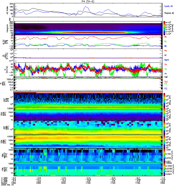
endObtain and analyze DC and AC wave data for an event, including wave polarization and Poynting flux. A whistler mode chorus event observed by THEMIS, occurred on TH-E (P5) at ~10:00-10:15 UT on 2008-12-15 (referenced in the class notes in Lecture 10, p.5) taken from the paper by Li et al., JGR 2011.
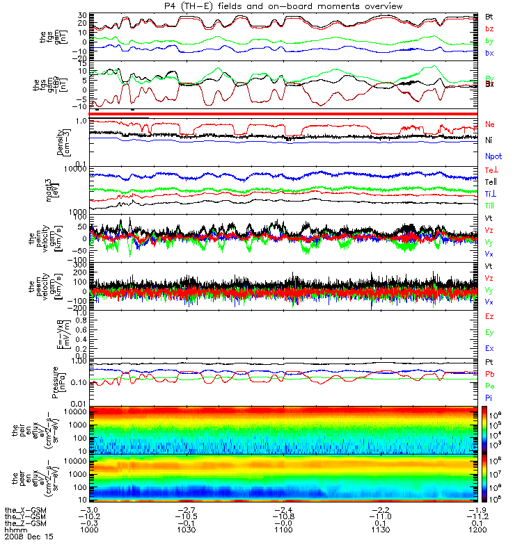
In the overview plots (here and here), E & B wavepower is significant during significant velocity oscillations. A different whistler mode chorus event was observed by MMS on 2019-08-16 at ~09:32:00UT within a flux pileup region shown in Fig. 2 of Fu et al., GRL 2025. MMS overview plot is here. Follow the structure of Hwk05_01.pro (just an example). Work in either IDL or PySPEDAS, for either the THEMIS or the MMS event to:
- Fig. 1. Identify the event in overview plots and point out the wave power related to it
- Fig. 2. Get the Electric Field (Double-Probe) Instruments (EFI) data, remove offsets, show ExB velocity, using E*B=0 approximation
- Fig. 3. Plot on-board computed spectra. Overplot fce, 1⁄2 fce
- Fig. 4. Recognize (wave)burst times in the waveforms and plot them and the spectra
- Fig. 5. Introduce E and B and show ground computed spectra (wavelet and Fourier)
- Fig. 6. Rotate into FAC coord’s and feed waveforms into wave analysis program. Plot results. Read the section of the relevant paper and explain the role/significance of the whistler waves in their respective setting.
- Fig. 7. Show the Poynting flux for the band-passed signal. Do this is time domain (process time series in real space) and in frequency domain (using the available tools).
Deliver a report explaining what you did, and your code.
Li et al. (2011)
We can clearly observe from the overview plot, specifically in the final panel, that the FBK exhibits wave activity within the frequency range of approximately 10–100 Hz. Additionally, it is evident that this wave activity is modulated with a period of roughly 10 seconds.
Similarly, the pressure, magnetic field, temperature, and electron density measurements also exhibit oscillations with a comparable period.
Get the Electric Field (Double-Probe) Instruments (EFI) data, remove offsets, show ExB velocity, using E*B=0 approximation
dir = "docs/courses/epss261/homework"
if isdir(dir)
cd(dir)
Pkg.activate(".")
Pkg.resolve()
Pkg.instantiate()
endusing Speasy
using CairoMakie
using Dates
using SpacePhysicsMakie
using LinearAlgebra
using Statistics
using DimensionalData
using Unitful
using PlasmaFormulary
using SignalAnalysis
using SPEDAS, TimeseriesUtilities
using Speasy: get_data
SpacePhysicsMakie.DEFAULTS.add_title = trueCondaPkg Found dependencies: /Users/zijin/.julia/packages/DimensionalData/FWnw9/CondaPkg.toml CondaPkg Found dependencies: /Users/zijin/.julia/packages/Speasy/zZJZI/CondaPkg.toml CondaPkg Found dependencies: /Users/zijin/.julia/packages/CondaPkg/0UqYV/CondaPkg.toml CondaPkg Found dependencies: /Users/zijin/.julia/packages/PythonCall/83z4q/CondaPkg.toml CondaPkg Found dependencies: /Users/zijin/.julia/packages/PySPEDAS/IGdx7/CondaPkg.toml CondaPkg Initialising pixi │ /Users/zijin/.julia/artifacts/d2fecc2a9fa3eac2108d3e4d9d155e6ff5dfd0b2/bin/pixi │ init │ --format pixi └ /Users/zijin/projects/beforerr/docs/courses/epss261/homework/.CondaPkg ✔ Created /Users/zijin/projects/beforerr/docs/courses/epss261/homework/.CondaPkg/pixi.toml CondaPkg Wrote /Users/zijin/projects/beforerr/docs/courses/epss261/homework/.CondaPkg/pixi.toml │ [dependencies] │ netcdf4 = "*" │ uv = ">=0.4" │ xarray = "*" │ sqlite = "!=3.49.1" │ numpy = "*" │ │ [dependencies.python] │ channel = "conda-forge" │ build = "*cp*" │ version = ">=3.10,!=3.14.0,!=3.14.1,<4, 3.13.*" │ │ [project] │ name = ".CondaPkg" │ platforms = ["osx-arm64"] │ channels = ["conda-forge"] │ channel-priority = "strict" │ description = "automatically generated by CondaPkg.jl" │ │ [pypi-dependencies.speasy] │ git = "https://github.com/SciQLop/speasy" │ │ [pypi-dependencies.pyspedas] └ git = "https://github.com/spedas/pyspedas" CondaPkg Installing packages │ /Users/zijin/.julia/artifacts/d2fecc2a9fa3eac2108d3e4d9d155e6ff5dfd0b2/bin/pixi │ install └ --manifest-path /Users/zijin/projects/beforerr/docs/courses/epss261/homework/.CondaPkg/pixi.toml WARN Using local manifest /Users/zijin/projects/beforerr/docs/courses/epss261/homework/.CondaPkg/pixi.toml rather than /Users/zijin/projects/beforerr/pyproject.toml from environment variable `PIXI_PROJECT_MANIFEST` ✔ The default environment has been installed. Precompiling packages... Info Given SPEDAS was explicitly requested, output will be shown live WARNING: Method definition name2dim(Base.Val{:𝑓}) in module PlasmaWavesDimensionalDataExt at /Users/zijin/.julia/packages/DimensionalData/FWnw9/src/Dimensions/dimension.jl:477 overwritten in module SPEDAS on the same line (check for duplicate calls to `include`). ERROR: Method overwriting is not permitted during Module precompilation. Use `__precompile__(false)` to opt-out of precompilation. 4563.6 ms ? SPEDAS WARNING: Method definition name2dim(Base.Val{:𝑓}) in module PlasmaWavesDimensionalDataExt at /Users/zijin/.julia/packages/DimensionalData/FWnw9/src/Dimensions/dimension.jl:477 overwritten in module SPEDAS on the same line (check for duplicate calls to `include`). ERROR: Method overwriting is not permitted during Module precompilation. Use `__precompile__(false)` to opt-out of precompilation.
truetrange_plus = ("2008-12-15T09:45:00", "2008-12-15T10:30:00")
trange = ("2008-12-15T09:55:00", "2008-12-15T10:20:00")("2008-12-15T09:55:00", "2008-12-15T10:20:00")"""
Reference: [SPEDAS](https://github.com/spedas/bleeding_edge/blob/master/idl/projects/themis/spacecraft/fields/thm_load_fit.pro)
"""
function thm_load_fit(probe, timerange; vars=["fgs_dsl", "efs_dsl", "efs_0_dsl", "efs_dot0_dsl"])
dataset = "TH$(uppercase(probe))_L2_FIT"
vars = "th$(lowercase(probe))_" .* vars
ids = "cda/$dataset/" .* vars
return map(DimArray, get_data(NamedTuple, ids, timerange))
end
data = thm_load_fit("e", trange)
tplot(data)Can't get THE_L2_FIT/the_fgs_dsl without web service, switching to web service
Can't get THE_L2_FIT/the_efs_dsl without web service, switching to web service
Can't get THE_L2_FIT/the_efs_0_dsl without web service, switching to web service
Can't get THE_L2_FIT/the_efs_dot0_dsl without web service, switching to web service
Here’s the Julia equivalent of the provided IDL code for removing offsets and calculating electric field components:
# Get Ez (dsl) and ExB
let B = data.the_fgs_dsl, E = data.the_efs_dsl, angle = 20.0 # degrees
# First get Ex/y offsets
println("Select 2 times (Start/Stop) for obtaining Ex, Ey offsets")
trange4offset = ["2008-12-15T10:30:00", "2008-12-15T10:40:00"]
data_offset = thm_load_fit("e", trange4offset)
Eoffsets = tmean(data_offset.the_efs_dsl)
@info "Eoffsets" Eoffsets.data
# Set angle threshold
tanangle = tan(angle * π / 180.0)
# Calculate the condition for each data point
B = B[DimSelectors(E)]
bxy_magnitude = sqrt.(B[:, 1] .^ 2 + B[:, 2] .^ 2)
angle_condition = abs.(B[:, 3] ./ bxy_magnitude) .>= tanangle
igood = findall(angle_condition)
ibad = findall(.!angle_condition)
janygood = length(igood)
janybad = length(ibad)
@info "janygood" janygood
@info "janybad" janybad
# Apply offsets to Ex and Ey components
E_corrected = copy(E)
E_corrected[:, 1] .-= Eoffsets[1]
E_corrected[:, 2] .-= Eoffsets[2]
# Set bad data points to NaN
if janybad >= 1
for i in ibad
E_corrected[i, :] .= NaN
end
end
if janygood < 1
println("*****WARNING: NO GOOD 3D ExB data")
else
for i in igood
E_corrected[i, 3] =
-(E_corrected[i, 1] * B[i, 1] +
E_corrected[i, 2] * B[i, 2]) /
B[i, 3]
end
end
f = Figure()
tplot(f[1, 1], data_offset)
tplot(f[1, 2:4], [B, E, E_corrected, data.the_efs_0_dsl, data.the_efs_dot0_dsl])
f
endSelect 2 times (Start/Stop) for obtaining Ex, Ey offsets Can't get THE_L2_FIT/the_fgs_dsl without web service, switching to web service Can't get THE_L2_FIT/the_efs_dsl without web service, switching to web service Can't get THE_L2_FIT/the_efs_0_dsl without web service, switching to web service Can't get THE_L2_FIT/the_efs_dot0_dsl without web service, switching to web service ┌ Info: Eoffsets │ Eoffsets.data = │ 3-element Vector{Float32}: │ -0.9041299 │ 0.07251182 └ -25.993834 ┌ Info: janygood └ janygood = 489 ┌ Info: janybad └ janybad = 0

In the left panel, we present the data utilized for the offset analysis. In the right panel, arranged sequentially from top to bottom, we display the magnetic field data, the electric field data, the electric field data corrected using our offset analysis, and finally, the corresponding electric field data extracted from the L2 dataset efs_0_dsl and efs_dot0_dsl.
let E = data.the_efs_dot0_dsl, B = data.the_fgs_dsl
B_int = tinterp(B, E)
V = tcross(E, B_int) ./ tdot(B_int, B_int) * 1000u"km/s"
V = setmeta(V, "LABLAXIS" => "Velocity", "UNITS" => "km/s"; labels=("Vx", "Vy", "Vz"))
tplot([B, E, V])
end
Computed \(V= E × B/B^2\) is shown in the last panel.
Plot on-board computed spectra. Overplot fce, 1⁄2 fce
function thm_load_fbk(probe, timerange; vars=("fb_edc12", "fb_scm1"))
dataset = "TH$(uppercase(probe))_L2_FBK"
vars = "th$(lowercase(probe))_" .* vars
ids = "cda/$dataset/" .* vars
DimArray.(get_data(ids, timerange))
end
thm_fb_edc12, thm_fb_scm1 = thm_load_fbk("e", trange)Can't get THE_L2_FBK/the_fb_edc12 without web service, switching to web service
Can't get THE_L2_FBK/the_fb_scm1 without web service, switching to web service2-element Vector{DimMatrix{Float32, Tuple{Ti{DimensionalData.Dimensions.Lookups.Sampled{UnixTimes.UnixTime, VariableAxis{UnixTimes.UnixTime, 1}, DimensionalData.Dimensions.Lookups.ForwardOrdered, DimensionalData.Dimensions.Lookups.Irregular{Tuple{Nothing, Nothing}}, DimensionalData.Dimensions.Lookups.Points, DimensionalData.Dimensions.Lookups.NoMetadata}}, Y{DimensionalData.Dimensions.Lookups.Sampled{Float32, VariableAxis{Float32, 1}, DimensionalData.Dimensions.Lookups.ReverseOrdered, DimensionalData.Dimensions.Lookups.Irregular{Tuple{Nothing, Nothing}}, DimensionalData.Dimensions.Lookups.Points, DimensionalData.Dimensions.Lookups.NoMetadata}}}, Tuple{}, PythonCall.PyArray{Float32, 2, true, false, Float32}, String, Speasy.OverlayDict{Union{String, Symbol}, Any}}}:
Float32[0.014709114 0.0073833982 … 0.012690215 0.01730484; 0.014709114 0.020304345 … 0.009229247 0.01730484; … ; 0.014709114 0.0 … 0.008075591 0.01730484; 0.0 0.0 … 0.013843872 0.020765807]
Float32[0.0032959487 0.00077439536 … 0.003418021 0.0085832; 0.0032959487 0.00077439536 … 0.0028839551 0.009536888; … ; 0.0032959487 0.00082780194 … 0.0023498894 0.0014305334; 0.00343328 0.00082780194 … 0.0024567025 0.0071526663]The three lines in Figures represent 1 fce (blue), 0.5 fce (orange), and 0.1 fce (green).
let B = tnorm(data.the_fgs_dsl) * 1u"nT"
fce = gyrofrequency.(B, :e) .|> ω2f
fce = setmeta(fce, scale=log10) ./ 1u"Hz"
f = tplot([thm_fb_edc12, thm_fb_scm1]; add_title=true, alpha=0.7)
tplot_panel!.(f.axes, Ref([fce, fce / 2, fce / 10]))
f
end
ffw_16_eac34 and ffp_16_eac34 ffp_16_scm3 data are not available for this event.
function thm_load_fft(probe, timerange; vars=("ffw_16_eac34", "ffp_16_eac34", "ffp_16_scm3"))
dataset = "TH$(uppercase(probe))_L2_FFT"
vars = "th$(lowercase(probe))_" .* vars
ids = "cda/$dataset/" .* vars
DimArray.(get_data(ids, timerange))
end
fft_tvars = [
"cda/THE_L2_FFT/the_ffp_16_eac34",
"cda/THE_L2_FFT/the_ffp_16_scm3",
"cda/THE_L2_FFT/the_ffw_16_eac34",
"cda/THE_L2_FFT/the_ffw_16_scm3",
]
fft_data = get_data.(fft_tvars, (trange,))
all(ismissing.(fft_data)) && @warn "Data not available"Can't get THE_L2_FFT/the_ffp_16_eac34 without web service, switching to web service
Can't get THE_L2_FFT/the_ffp_16_scm3 without web service, switching to web service
Can't get THE_L2_FFT/the_ffw_16_eac34 without web service, switching to web service
Can't get THE_L2_FFT/the_ffw_16_scm3 without web service, switching to web servicefalseRecognize (wave)burst times in the waveforms and plot them and the spectra.
tvars = [
"cda/THE_L2_SCM/the_scp_dsl",
"cda/THE_L2_SCM/the_scw_dsl",
]
thm_scp_dsl, thm_scw_dsl = get_data.(tvars, (trange_plus,)) .|> DimArray
f = Figure()
tplot(f[1, 1], [thm_scp_dsl, thm_scw_dsl])
fCan't get THE_L2_SCM/the_scp_dsl without web service, switching to web service
Can't get THE_L2_SCM/the_scw_dsl without web service, switching to web service
We see a waveburst around 2008-12-15T10:13:10.
tvars_wb = [
"cda/THE_L2_SCM/the_scp_dsl",
"cda/THE_L2_SCM/the_scw_dsl",
"cda/THE_L2_FBK/the_fb_scm1",
]
trange_wb = DateTime.(("2008-12-15T10:13:10", "2008-12-15T10:13:20"))
trange_wb_s = ("2008-12-15T10:13:10", "2008-12-15T10:13:17")
data_wb = get_data.(tvars_wb, (trange_wb,)) .|> DimArray
# tplot(f[1, 2], data_wb)
tplot(f[1, 2], data_wb)
tlims!(trange_wb_s)
fCan't get THE_L2_SCM/the_scp_dsl without web service, switching to web service
Can't get THE_L2_SCM/the_scw_dsl without web service, switching to web service
Can't get THE_L2_FBK/the_fb_scm1 without web service, switching to web service
Introduce E and B and show ground computed spectra (wavelet and Fourier)
using PySPEDAS.Projects
thm_efi_ds = themis.efi(trange, level="l1", probe="e")
thm_efw = DimArray(thm_efi_ds.the_efw)Loading efw data using PySPEDAS is somehow quite slow, instead we define a configuration file and load the efw data from the SPDF.
the_efw_l1:
inventory_path: spdf/THEMIS/THE/L1/EFW
master_cdf: https://spdf.gsfc.nasa.gov/pub/data/themis/the/l1/efw/2021/the_l1_efw_20210102_v01.cdf
split_frequency: daily
split_rule: regular
url_pattern: https://spdf.gsfc.nasa.gov/pub/data/themis/the/l1/efw/{Y}/the_l1_efw_{Y}{M:02d}{D:02d}_v\d+.cdf
use_file_list: truethe_efw_l1_index = speasy.inventories.data_tree.archive.spdf.THEMIS.THE.L1.EFW.the_efw_l1
tvars = [
"cda/THE_L2_FGM/the_fgs_gsm",
"cda/THE_L2_FGM/the_fgh_gsm",
"cda/THE_L2_SCM/the_scp_dsl",
"cda/THE_L2_SCM/the_scw_dsl"
]
thm_fgs_gsm, thm_fgh_gsm, thm_scp_dsl, thm_scw_dsl = get_data(tvars, trange_plus) .|> DimArrayCan't get THE_L2_FGM/the_fgs_gsm without web service, switching to web service
Can't get THE_L2_FGM/the_fgh_gsm without web service, switching to web service
Can't get THE_L2_SCM/the_scp_dsl without web service, switching to web service
Can't get THE_L2_SCM/the_scw_dsl without web service, switching to web service4-element Vector{DimMatrix{Float32, Tuple{Ti{DimensionalData.Dimensions.Lookups.Sampled{UnixTimes.UnixTime, VariableAxis{UnixTimes.UnixTime, 1}, DimensionalData.Dimensions.Lookups.ForwardOrdered, DimensionalData.Dimensions.Lookups.Irregular{Tuple{Nothing, Nothing}}, DimensionalData.Dimensions.Lookups.Points, DimensionalData.Dimensions.Lookups.NoMetadata}}, Y{DimensionalData.Dimensions.Lookups.Sampled{Int32, VariableAxis{Int32, 1}, DimensionalData.Dimensions.Lookups.ForwardOrdered, DimensionalData.Dimensions.Lookups.Irregular{Tuple{Nothing, Nothing}}, DimensionalData.Dimensions.Lookups.Points, DimensionalData.Dimensions.Lookups.NoMetadata}}}, Tuple{}, PythonCall.PyArray{Float32, 2, true, false, Float32}, String, Speasy.OverlayDict{Union{String, Symbol}, Any}}}:
Float32[-6.884452 2.770554 13.2441; -6.8816504 2.699388 13.368085; … ; -10.854679 -2.0566497 25.193708; -11.012929 -1.8605247 25.144516]
Float32[-4.202244 1.5139444 15.179175; -4.1365685 1.664007 15.140432; … ; -8.527703 -0.975849 22.252335; -8.648017 -1.0026835 22.07751]
Float32[-7.3053866f-6 -1.8908788f-5 -2.836187f-5; -7.3053866f-6 -1.8908788f-5 -2.836187f-5; … ; 4.3625614f-6 5.230054f-6 -9.406129f-6; 4.3625614f-6 5.230054f-6 -9.406129f-6]
Float32[-0.000119733224 0.00037838318 -0.00024678188; -0.000119733224 0.00037838318 -0.00024678188; … ; 0.0017912713 -0.0006972916 0.0004022404; 0.0017912713 -0.0006972916 0.0004022404]thm_fgs_gsm_z_dpwrspc = SPEDAS.pspectrum(thm_fgs_gsm[:, 3]; nfft=64) |> SpacePhysicsMakie.set_colorrange!
thm_scp_dsl_z_dpwrspc = SPEDAS.pspectrum(thm_scp_dsl[:, 3]; nfft=512) |> SpacePhysicsMakie.set_colorrange!
thm_fgh_gsm_z_dpwrspc = SPEDAS.pspectrum(thm_fgh_gsm[:, 3]) |> SpacePhysicsMakie.set_colorrange!
# SpaceTools.set_colorrange
tvars_wb = [
the_efw_l1_index.the_efw,
"cda/THE_L2_SCM/the_scw_dsl"
]
thm_efw, thm_scw_dsl = get_data.(tvars_wb, (trange_wb,)) .|> DimArray
thm_scw_dsl_z_dpwrspc = SPEDAS.pspectrum(thm_scw_dsl[:, 3]) |> SpacePhysicsMakie.set_colorrange!
thm_efw_z_dpwrspc = SPEDAS.pspectrum(thm_efw[:, 3]) |> SpacePhysicsMakie.set_colorrange!
f = Figure()
tplot(f[1, 1], [
thm_fgs_gsm, thm_fgs_gsm_z_dpwrspc,
thm_fgh_gsm, thm_fgh_gsm_z_dpwrspc,
thm_scp_dsl, thm_scp_dsl_z_dpwrspc,
])
tplot(f[1, 2], [
thm_scw_dsl, thm_scw_dsl_z_dpwrspc,
thm_efw, thm_efw_z_dpwrspc,
])┌ Warning: Time resolution is is not approximately constant (relerr ≈ 511.0) └ @ TimeseriesUtilities ~/.julia/dev/TimeseriesUtilities/src/timeseries.jl:5 ┌ Warning: Time resolution is is not approximately constant (relerr ≈ 512.0) └ @ TimeseriesUtilities ~/.julia/dev/TimeseriesUtilities/src/timeseries.jl:5 Can't get THE_L2_SCM/the_scw_dsl without web service, switching to web service ┌ Warning: Time resolution is is not approximately constant (relerr ≈ 0.0020964360587002098) └ @ TimeseriesUtilities ~/.julia/dev/TimeseriesUtilities/src/timeseries.jl:5

During the interval when we have wavebursts, the whistle wave is clearly identifiable in the SCP data. However, in the higher-frequency data product, it becomes difficult to discern any distinct signatures within the spectrogram.
Rotate into FAC coord’s and feed waveforms into wave analysis program. Plot results. Read the section of the relevant paper and explain the role/significance of the whistler waves in their respective setting.
tvars = [
"cda/THE_L2_FGM/the_fgs_dsl",
"cda/THE_L2_FGM/the_fgh_dsl",
"cda/THE_L2_SCM/the_scp_dsl",
]
_trange = ["2008-12-15T09:59", "2008-12-15T10:13"]
thm_fgs_dsl, thm_fgh_dsl, thm_scp_dsl = Speasy.get_data(tvars, _trange) .|> DimArray
fac_mats = tfac_mat(thm_fgs_dsl)
thm_scp_fac = select_rotate(thm_scp_dsl, fac_mats, "FAC")
thm_fgh_fac = select_rotate(thm_fgh_dsl, fac_mats, "FAC")
f = Figure()
tplot(f[1, 1], [
thm_fgs_dsl,
thm_fgh_dsl,
thm_scp_dsl,
])
tplot(f[1, 2], [
thm_fgh_fac,
thm_scp_fac,
])Can't get THE_L2_FGM/the_fgs_dsl without web service, switching to web service Can't get THE_L2_FGM/the_fgh_dsl without web service, switching to web service Can't get THE_L2_SCM/the_scp_dsl without web service, switching to web service ┌ Warning: (DimensionalData.Dimensions.Y,) dims were not found in object. └ @ DimensionalData.Dimensions ~/.julia/packages/DimensionalData/FWnw9/src/Dimensions/primitives.jl:852 ┌ Warning: (DimensionalData.Dimensions.Y,) dims were not found in object. └ @ DimensionalData.Dimensions ~/.julia/packages/DimensionalData/FWnw9/src/Dimensions/primitives.jl:852

f = Figure(;)
tplot(f[1, 1], thm_fgh_fac)
tplot(f[2:6, 1], twavpol(tresample(thm_fgh_fac)))
tplot(f[1, 2], thm_scp_fac)
tplot(f[2:6, 2], twavpol(tresample(thm_scp_fac)))┌ Warning: Time resolution is is not approximately constant (relerr ≈ 512.0) └ @ TimeseriesUtilities ~/.julia/dev/TimeseriesUtilities/src/timeseries.jl:5

Compressional pulsations are associated with modulations of resonant electron fluxes and chorus intensity.
We have developed a high-performance wave polarization program implemented in Julia, achieving a significant speedup of approximately 100 times compared to its Python counterpart. Furthermore, our implementation is more generalizable, extending the original program’s capabilities to accommodate data in n dimensions. The program is accessible via the following link:
Core part is attached in the appendix.
From top to bottom, we present the original data, the cleaned data with spikes removed, and the filtered data.
The right panel provides a magnified view of the data presented in the left panel
We can see that removing spikes is essential for the accuracy of the filtered data.
using TimeseriesUtilities: tfilter
begin
window = 128
E = Float64.(tclip(thm_efw, trange_wb))
E_clean = replace_outliers(E; window)
E_sm = tfilter(E, 64u"Hz")
E_clean_sm = tfilter(tinterp_nans(E_clean), 64u"Hz")
tvars = [E, E_clean, E_sm, E_clean_sm] .|> tshift
f = Figure()
tplot(f[1, 1], tvars)
fa2 = tplot(f[1, 2], tvars; link_yaxes=true)
t0 = E_clean |> tminimum
tlims!.(fa2.axes, 3.44u"s", 3.48u"s")
f
end┌ Warning: Time resolution is is not approximately constant (relerr ≈ 0.0020964360587002098) └ @ TimeseriesUtilities ~/.julia/dev/TimeseriesUtilities/src/timeseries.jl:5 ┌ Warning: Time resolution is is not approximately constant (relerr ≈ 0.0020964360587002098) └ @ TimeseriesUtilities ~/.julia/dev/TimeseriesUtilities/src/timeseries.jl:5 ┌ Warning: Time resolution is is not approximately constant (relerr ≈ 0.0020964360587002098) └ @ TimeseriesUtilities ~/.julia/dev/TimeseriesUtilities/src/timeseries.jl:5 ┌ Warning: Time resolution is is not approximately constant (relerr ≈ 0.0020964360587002098) └ @ TimeseriesUtilities ~/.julia/dev/TimeseriesUtilities/src/timeseries.jl:5

Poynting_vector(E, B) = setmeta(tcross(E, B) ./ Unitful.μ0, "LABL_PTR_1" => ["Sx", "Sy", "Sz"], "UNITS" => "nW/m^2")
begin
B = tclip(thm_scw_dsl, trange_wb)
E = Float64.(tclip(thm_efw, trange_wb))
B = B[DimSelectors(E; selectors=Near())]
E_clean = replace_outliers(E; window=128)
B_sm = tfilter(B, 64u"Hz")
E_clean_sm = tfilter(tinterp_nans(E_clean), 64u"Hz")
S = Poynting_vector(B, E)
S_sm = Poynting_vector(B_sm, E_clean_sm)
f = Figure()
tplot(f[1, 1:2], [thm_scw_dsl, thm_efw])
tplot(f[2:4, 1], [B, E, S])
tplot(f[2:4, 2], [B_sm, E_clean_sm, S_sm])
f
end┌ Warning: Time resolution is is not approximately constant (relerr ≈ 1.0) └ @ TimeseriesUtilities ~/.julia/dev/TimeseriesUtilities/src/timeseries.jl:5 ┌ Warning: Time resolution is is not approximately constant (relerr ≈ 1.0) └ @ TimeseriesUtilities ~/.julia/dev/TimeseriesUtilities/src/timeseries.jl:5 ┌ Warning: Time resolution is is not approximately constant (relerr ≈ 0.0020964360587002098) └ @ TimeseriesUtilities ~/.julia/dev/TimeseriesUtilities/src/timeseries.jl:5 ┌ Warning: Time resolution is is not approximately constant (relerr ≈ 0.0020964360587002098) └ @ TimeseriesUtilities ~/.julia/dev/TimeseriesUtilities/src/timeseries.jl:5

From top to bottom, the panels show the Poynting flux and its corresponding frequency spectra in the x, y, z directions and magnitude, respectively.
let S = tnorm_combine(S_sm)
S_dpwrspc = pspectrum(S; nfft=512) |> SpacePhysicsMakie.set_colorrange!
f = tplot([
S,
eachslice(S_dpwrspc; dims=Y())...
])
end┌ Warning: Time resolution is is not approximately constant (relerr ≈ 1.0) └ @ TimeseriesUtilities ~/.julia/dev/TimeseriesUtilities/src/timeseries.jl:5 ┌ Warning: Time resolution is is not approximately constant (relerr ≈ 1.0) └ @ TimeseriesUtilities ~/.julia/dev/TimeseriesUtilities/src/timeseries.jl:5 ┌ Warning: Time resolution is is not approximately constant (relerr ≈ 1.0) └ @ TimeseriesUtilities ~/.julia/dev/TimeseriesUtilities/src/timeseries.jl:5 ┌ Warning: Time resolution is is not approximately constant (relerr ≈ 1.0) └ @ TimeseriesUtilities ~/.julia/dev/TimeseriesUtilities/src/timeseries.jl:5

Core codes is pasted here for reference (which is readable to some extent:).
"""
spectral_matrix(X, window)
"""
function spectral_matrix(X::AbstractMatrix, window::AbstractVector=ones(size(X, 1)))
n_samples, n = size(X)
# Apply the window to each component
Xw = X .* window
# Compute FFTs and normalize
Xf = fft(Xw, 1) ./ sqrt(n_samples)
# Only keep the positive frequencies
Nfreq = div(n_samples, 2)
Xf = Xf[1:Nfreq, :]
S = Array{ComplexF64,3}(undef, Nfreq, n, n)
for i in 1:n, j in 1:n
@. S[:, i, j] = Xf[:, i] * conj(Xf[:, j])
end
return S
end
"""
wavpol(ct, X; nfft=256, noverlap=nfft÷2, bin_freq=3)
Perform polarization analysis of `n`-component time series data.
Assumes the data are in a right-handed, field-aligned coordinate system
(with Z along the ambient magnetic field).
For each FFT window (with specified overlap), the routine:
1. Computes the FFT and constructs the spectral matrix ``S(f)``.
2. Applies frequency smoothing using a window (of length `bin_freq`).
3. Computes the wave power, degree of polarization, wave normal angle,
ellipticity, and helicity.
# Returns
A tuple: where each parameter (except `freqline`) is an array with one row per FFT window.
"""
function wavpol(ct, X; nfft=256, noverlap=div(nfft, 2), bin_freq=3)
# Ensure the smoothing window length is odd.
iseven(bin_freq) && (bin_freq += 1)
N = size(X, 1)
samp_freq = samplingrate(ct)
Nfreq = div(nfft, 2)
fs = (samp_freq / nfft) * (0:(Nfreq-1))
# Define the number of FFT windows and times (center time of each window)
nsteps = floor(Int, (N - nfft) / noverlap) + 1
times = similar(ct, nsteps)
# Define the FFT window (here a smooth window similar to Hanning)
window = 0.08 .+ 0.46 .* (1 .- cos.(2π .* (0:(nfft-1)) ./ nfft))
half = div(nfft, 2)
# Use a Hamming window for frequency smoothing.
smooth_win = 0.54 .- 0.46 * cos.(2π .* (0:(bin_freq-1)) ./ (bin_freq - 1))
smooth_win = smooth_win / sum(smooth_win)
# Preallocate arrays for the results.
power = zeros(Float64, nsteps, Nfreq)
degpol = zeros(Float64, nsteps, Nfreq)
waveangle = zeros(Float64, nsteps, Nfreq)
ellipticity = zeros(Float64, nsteps, Nfreq)
helicity = zeros(Float64, nsteps, Nfreq)
# Process each FFT window.
Threads.@threads for j in 1:nsteps
start_idx = 1 + (j - 1) * noverlap
end_idx = start_idx + nfft - 1
if end_idx > N
continue
end
S = spectral_matrix(@view(X[start_idx:end_idx, :]), window)
S_smooth = smooth_spectral_matrix(S, smooth_win)
params = compute_polarization_parameters(S_smooth)
# Store the results.
power[j, :] = params.power
degpol[j, :] = params.degpol
waveangle[j, :] = params.waveangle
ellipticity[j, :] = params.ellipticity
helicity[j, :] = params.helicity
times[j] = ct[start_idx+half] # Set the times at the center of the FFT window.
end
return (; times, fs, power, degpol, waveangle, ellipticity, helicity)
endfunction wpol_helicity(S::AbstractMatrix{ComplexF64}, waveangle::Number)
# Preallocate arrays for 3 polarization components
helicity_comps = zeros(Float64, 3)
ellip_comps = zeros(Float64, 3)
for comp in 1:3
# Build state vector λ_u for this polarization component
alph = sqrt(real(S[comp, comp]))
alph == 0.0 && continue
if comp == 1
lam_u = [
alph,
(real(S[1, 2]) / alph) + im * (-imag(S[1, 2]) / alph),
(real(S[1, 3]) / alph) + im * (-imag(S[1, 3]) / alph)
]
elseif comp == 2
lam_u = [
(real(S[2, 1]) / alph) + im * (-imag(S[2, 1]) / alph),
alph,
(real(S[2, 3]) / alph) + im * (-imag(S[2, 3]) / alph)
]
else
lam_u = [
(real(S[3, 1]) / alph) + im * (-imag(S[3, 1]) / alph),
(real(S[3, 2]) / alph) + im * (-imag(S[3, 2]) / alph),
alph
]
end
# Compute the phase rotation (gammay) for this state vector
lam_y = phase_factor(lam_u) * lam_u
# Helicity: ratio of the norm of the imaginary part to the real part
norm_real = norm(real(lam_y))
norm_imag = norm(imag(lam_y))
helicity_comps[comp] = (norm_imag != 0) ? norm_imag / norm_real : NaN
# For ellipticity, use only the first two components
u1 = lam_y[1]
u2 = lam_y[2]
# TODO: why there is no 2 in front of uppere?
uppere = imag(u1) * real(u1) + imag(u2) * real(u2)
lowere = (-imag(u1)^2 + real(u1)^2 - imag(u2)^2 + real(u2)^2)
gammarot = atan(uppere, lowere)
lam_urot = exp(-1im * 0.5 * gammarot) * [u1, u2]
num = norm(imag(lam_urot))
den = norm(real(lam_urot))
ellip_val = (den != 0) ? num / den : NaN
# Adjust sign using the off-diagonal of ematspec and the wave normal angle
sign_factor = sign(imag(S[1, 2]) * sin(waveangle))
ellip_comps[comp] = ellip_val * sign_factor
end
# Average the three computed values
helicity = mean(helicity_comps)
ellipticity = mean(ellip_comps)
return helicity, ellipticity
endSearch Coil Magnetometer (SCM) science data
WB waveforms (scw) [8192 S/s]
https://themis.igpp.ucla.edu/scm_dataflow.shtml
Electric Field Instruments (EFI) science data
PB waveforms (efp, vap) [128 S/s; Allocation ~ 1.2h]
WB waveforms (efw, vaw) [8192 S/s; Allocation ~ 43s]
https://themis.ssl.berkeley.edu/instrument_efi.shtml