Overview of the event

We are using PSP_SWP_SPI_SF00_L3_MOM dataset

DSCOVR_H1_FC/Np outside of its definition range <DateTimeRange: 2016-06-03T00:00:00+00:00 -> 2019-06-27T23:58:59+00:00>

# hvplot.extension('bokeh', 'matplotlib')
# hvplot.output(backend='matplotlib', fig='svg')

psp_dataset = "PSP_SWP_SPI_SF00_L3_MOM"
psp_parameters = ["DENS", "VEL_RTN_SUN", "TEMP", "MAGF_SC", "SUN_DIST"]

# Encounter 2
psp_start = "2019-04-07T01:00"
psp_end = "2019-04-07T09:00"

earth_start = "2019-04-09"
earth_end = "2019-04-14"

every = timedelta(minutes=4)

mission = "Wind"
# mission = "DSCOVR"

fname = f"../figures/evolution/plasma-adiabatic-evolution_e2-{mission}"

# # Encounter 4
# psp_start = '2020-01-27'
# psp_end = '2020-01-29'

# earth_start = '2020-01-29'
# earth_end = '2020-01-31'

# every = timedelta(minutes=4)

# mission = 'Wind'

# fname = f"../figures/evolution/plasma-adiabatic-evolution_e4-{mission}"

psp_timerange = TimeRange(psp_start, psp_end)

earth_timerange = TimeRange(earth_start, earth_end)

match mission.lower():
    case "dscovr":
        e_mag_dataset = "DSCOVR_H0_MAG"
        e_mag_parameters = ["B1F1"]
        e_plasma_dataset = "DSCOVR_H1_FC"
        e_plasma_parameters = ["Np", "V_GSE", "THERMAL_TEMP"]
    case "wind":
        e_mag_dataset = "WI_K0_MFI"
        e_mag_parameters = ["BF1"]
        e_plasma_dataset = "WI_K0_SWE"
        e_plasma_parameters = ["Np", "V_GSM", "THERMAL_SPD"]

def validate(timerange):
    if isinstance(timerange, TimeRange):
        return [timerange.start.to_string(), timerange.end.to_string()]

psp_plasma_vars = Variables(
    dataset=psp_dataset, parameters=psp_parameters, timerange=validate(psp_timerange)
).retrieve_data()

vec_cols = psp_plasma_vars.data[1].columns
psp_mag_cols = psp_plasma_vars.data[3].columns

def preview(products: list[str]):
    vars = Variables(
        products=products, timerange=validate(earth_timerange)
    ).retrieve_data()

    fig, axes = plt.subplots(2)
    vars.data[0].replace_fillval_by_nan().plot(ax=axes[0])
    vars.data[1].replace_fillval_by_nan().plot(ax=axes[1])

    return fig, axes


# preview(["cda/DSCOVR_H1_FC/THERMAL_TEMP", "cda/WI_K0_SWE/THERMAL_SPD"])
# preview(["cda/DSCOVR_H0_MAG/B1F1", "cda/WI_K0_MFI/BF1"])

vars = Variables(
    products=["cda/DSCOVR_H1_FC/THERMAL_TEMP", "cda/WI_K0_SWE/THERMAL_SPD"],
    timerange=validate(earth_timerange),
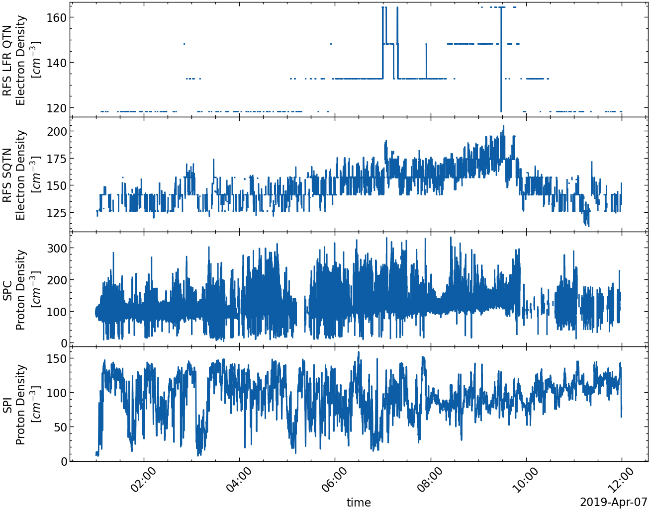
).retrieve_data()

Check Different Density Product

Time resolution (from high to low): SPC, SPI, SQTN, QTN Quality (fluctuating, from high to low): SQTN, QTN, SPC/SPI

So we use SQTN dataset for density variables.

from space_analysis.utils.speasy import Variables, Variable

vs = Variables(
    timerange=psp_timerange,
    variables=[
        Variable(
            product="cda/PSP_FLD_L3_RFS_LFR_QTN/N_elec",
            name="RFS LFR QTN\nElectron Density\n[$cm^{{-3}}$]",
        ),
        Variable(
            product="cda/PSP_FLD_L3_SQTN_RFS_V1V2/electron_density",
            name="RFS SQTN\nElectron Density\n[$cm^{{-3}}$]",
        ),
        Variable(
            product="cda/PSP_SWP_SPC_L3I/np_moment_gd",
            name="SPC\nProton Density\n[$cm^{{-3}}$]",
        ),
        Variable(
            product="cda/PSP_SWP_SPI_SF00_L3_MOM/DENS",
            name="SPI\nProton Density\n[$cm^{{-3}}$]",
        ),
    ],
)

fig, axes = vs.plot()
fig.set_size_inches(15, 12)
# remove legend from all
for ax in axes:
    ax.get_legend().remove()

fig.savefig(
    "../figures/examples/psp_density_comparison.png", bbox_inches="tight", dpi=300
)

from speasy import get_data, SpeasyVariable

def check_time_resolution(timerange, products: list[str]):
    data = get_data(products, timerange)

    data: list[SpeasyVariable]

    for d in data:
        df = pl.from_dataframe(
            d.replace_fillval_by_nan()
            .to_dataframe()
            .reset_index()
            .rename(columns={"index": "time"})
        )

        info = df.with_columns(delta=pl.col("time").diff()).describe()

        info_clean = df.drop_nulls().select(delta=pl.col("time").diff()).describe()

        display(info.join(info_clean, on="statistic", suffix=" (clean)"))

Figure 1

Radial evolution of the coronal hole high-speed streams

Perrone et al. (2019) used HELIOS observations to study the radial evolution of the solar wind in coronal hole high-speed streams. They found that The radial dependence of the proton number density, np, and the magnetic field, B, is given by

The radial dependence of the proton number density, np is

\[n_p = (2.4 ± 0.1)(R/R_0)^{−(1.96±0.07)} cm^{−3}\]

\[B = (5.7 ± 0.2)(R/R_0)^{−(1.59±0.06)} nT\]

The faster decrease of the magnetic than kinetic pressure is reflected in the radial proton plasma beta variation

\[β_p = P_k/P_B = (0.55 ± 0.04)(R/R_0)^{(0.4±0.1)}.\]

The behaviour of the parallel proton plasma beta is similar

\[β_{‖} = (0.37 ± 0.03)(R/R_0)^{(0.8±0.1)}\]

def plasma_r_evolution(
    df: pl.DataFrame,
    alpha_beta_r=0.4,
    alpha_beta_parallel_r=0.9,
    alpha_n=-2,
    alpha_B=-1.63,
    alpha_plasma_speed=0,
):
    return df.with_columns(
        plasma_speed_1AU=pl.col("plasma_speed")
        * (1 / pl.col("distance2sun")) ** alpha_plasma_speed,
        n_1AU=pl.col("n") * (1 / pl.col("distance2sun")) ** alpha_n,
        B_1AU=pl.col("B") * (1 / pl.col("distance2sun")) ** alpha_B,
        beta_1AU=pl.col("beta") * (1 / pl.col("distance2sun")) ** alpha_beta_r,
        beta_parallel=pl.col("beta")
        * (1 / pl.col("distance2sun")) ** alpha_beta_parallel_r,
    )

km2au = u.km.to(u.AU)

psp_plasma_r = (
    psp_plasma_vars.to_polars()
    .pipe(resample, every)
    .with_columns(
        B=pl_norm(psp_mag_cols),
        plasma_speed=pl_norm(vec_cols),
        distance2sun=pl.col("Sun Distance") * km2au,
    )
    .rename(
        {
            "Density": "n",
            "Temperature": "T",
        }
    )
    .collect()
    .pipe(df_beta)
    .pipe(plasma_r_evolution)
    .pipe(df_Alfven_speed)
    .pipe(df_Alfven_speed, B="B_1AU", n="n_1AU", col_name="Alfven_speed_1AU")
    .with_columns(
        plasma_speed_over_Alfven_speed=pl.col("plasma_speed") / pl.col("Alfven_speed"),
        plasma_speed_over_Alfven_speed_1AU=pl.col("plasma_speed_1AU")
        / pl.col("Alfven_speed_1AU"),
    )
)

def thermal_spd2temp(speed, speed_unit=u.km / u.s):
    return (m_p * (speed * speed_unit) ** 2 / 2).to("eV").value


def df_thermal_spd2temp(
    ldf: pl.LazyFrame,
    speed_col,
    speed_unit=u.km / u.s,
    name="plasma_temperature",
    temp_unit=u.eV,
):
    df = ldf.collect()
    temp = thermal_spd2temp(df[speed_col].to_numpy(), speed_unit)
    return df.with_columns(pl.Series(temp).alias(name)).lazy()

def process(
    timerange,
    mag_dataset: str,
    mag_parameters: list[str],
    plasma_dataset: str,
    plasma_parameters: list[str],
):
    timerange = validate(timerange)

    mag_vars = Variables(
        dataset=mag_dataset,
        parameters=mag_parameters,
        timerange=timerange,
    ).retrieve_data()

    plasma_vars = Variables(
        dataset=plasma_dataset,
        parameters=plasma_parameters,
        timerange=timerange,
    ).retrieve_data()

    temp_vars = plasma_vars.data[2]

    density_col = plasma_vars.data[0].columns[0]
    vec_cols = plasma_vars.data[1].columns
    temp_col = temp_vars.columns[0]
    mag_col = mag_vars.data[0].columns[0]

    plasma_data = (
        plasma_vars.to_polars()
        .with_columns(plasma_speed=pl_norm(vec_cols))
        .rename({density_col: "n"})
    ).pipe(resample, every)
    # process temperature data

    if temp_vars.unit == "km/s":
        plasma_data = plasma_data.pipe(df_thermal_spd2temp, temp_col, name="T")
        T_unit = u.eV
    else:
        plasma_data = plasma_data.rename({temp_col: "T"})
        if temp_vars.unit.startswith("K"):
            T_unit = u.K

    mag_data = mag_vars.to_polars().pipe(resample, every).rename({mag_col: "B"})

    df = (
        plasma_data.sort("time")
        .join_asof(mag_data.sort("time"), on="time")
        .collect()
        .pipe(df_beta, T_unit=T_unit)
        .pipe(df_Alfven_speed)
        .with_columns(
            plasma_speed_over_Alfven_speed=pl.col("plasma_speed")
            / pl.col("Alfven_speed"),
        )
    )
    return df

from copy import deepcopy

func = partial(
    process,
    mag_dataset=e_mag_dataset,
    mag_parameters=e_mag_parameters,
    plasma_dataset=e_plasma_dataset,
    plasma_parameters=e_plasma_parameters,
)

e_df_previous = func(deepcopy(earth_timerange).previous())
e_df = func(earth_timerange)
e_df_next = func(deepcopy(earth_timerange).next())

plot = psp_plasma_r.plot(
    x="time",
    y=["plasma_speed", "beta", "Alfven_speed", "plasma_speed_over_Alfven_speed"],
    subplots=True,
    shared_axes=False,
).cols(1)

plot_1AU = psp_plasma_r.plot(
    x="time",
    y=[
        "plasma_speed_1AU",
        "beta_1AU",
        "Alfven_speed_1AU",
        "plasma_speed_over_Alfven_speed_1AU",
    ],
    subplots=True,
    shared_axes=False,
).cols(1)

plot + plot_1AU

Cannot render NdLayout nested inside a Layout

:Layout
   .NdLayout.I  :NdLayout   [Variable]
      :Curve   [time]   (value)
   .NdLayout.II :NdLayout   [Variable]
      :Curve   [time]   (value)

def compare_df(df1, df2):
    df1_plot = df1.plot.scatter(
        x="beta", y="plasma_speed_over_Alfven_speed", label="PSP"
    ) * df1.plot.scatter(
        x="beta_1AU",
        y="plasma_speed_over_Alfven_speed_1AU",
        label="PSP (1AU predicted)",
    )

    df2_plot = df2.plot.scatter(
        x="beta",
        y="plasma_speed_over_Alfven_speed",
        label=mission,
        alpha=0.2,
    )

    xlabel = "Plasma beta"
    # ylabel=r"$v_i$ / $v_A$"
    ylabel = "Plasma speed over Alfven speed"

    return (df2_plot * df1_plot).opts(
        xlabel=xlabel, ylabel=ylabel, logx=True, logy=True
    )

hvplot.extension("bokeh", "matplotlib")
hvplot.output(backend="matplotlib", fig="svg")

fig = compare_df(psp_plasma_r, e_df_previous).opts(title="Previous Period")
hvplot.save(fig, fname + "-previous", fmt="svg")
# hvplot.save(fig, fname + "-previous.svg")

fig = compare_df(psp_plasma_r, e_df).opts(title="Current Period")
hvplot.save(fig, fname, fmt="svg")

fig = compare_df(psp_plasma_r, e_df_next).opts(title="Next Period")
hvplot.save(fig, fname + "-next", fmt="svg")

Datetime slider

import panel as pn

datetime_range_slider = pn.widgets.DatetimeRangeSlider(
    name="Datetime Range Slider",
    start=datetime(2017, 1, 1),
    end=datetime(2019, 1, 1),
    value=(datetime(2017, 1, 1), datetime(2018, 1, 10)),
    step=10000,
)

datetime_range_slider

References

Perrone, Denise, D Stansby, T S Horbury, and L Matteini. 2019. “Radial Evolution of the Solar Wind in Pure High-Speed Streams: HELIOS Revised Observations.” Monthly Notices of the Royal Astronomical Society 483 (3): 3730–37. https://doi.org/10.1093/mnras/sty3348.