Multifluid model of a one-dimensional steady state force-free current sheet
Introduction
Motivation
In MHD theory, for rotational rotational discontinuity, we have this following relationship
\[ [[\vec{U}]]=\left(\frac{\xi \rho}{\mu_0}\right)^{1 / 2}\left[\left[\frac{\vec{B}}{\rho}\right]\right] \]
where \(\xi \equiv 1-\frac{p_{\parallel}-p_{\perp}}{B^2 / \mu_0}\).
However, observations of solar wind discontinuities reveals discrepancies between
- Alfven velocity and plasma velocity change across discontinuities
- Anisotropic MHD theory-predicted and directly measured ion anisotropies
Multifluid theory is proposed to address these discrepancies. The basic idea is that we could have zero bulk velocity with non zero pressure.
MHD in a nutshell
\[ \begin{aligned} & \frac{\partial \rho}{\partial t}+(\vec{V} \cdot \nabla) \rho+\rho \nabla \cdot \vec{V}=0 \\ & \rho\left[\frac{\partial \vec{V}}{\partial t}+(\vec{V} \cdot \nabla) \vec{V}\right]+\nabla p=\vec{J} \times \vec{B} \\ & p=\alpha \rho^\gamma \\ & \nabla \times \vec{B}=\mu_0 \vec{J} \\ & \frac{\partial \vec{B}}{\partial t}=\nabla \times(\vec{V} \times \vec{B}) \end{aligned} \]
Previous Work
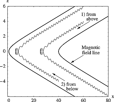
On the extreme of multiple fluid theory, we have the kinetic Harris model for the current sheet.
- no normal field, \(B_z = 0\)
- uniform cross-tail drift velocity, \(u_y\)
- vanishing particle density far from the sheet
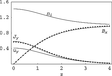
Steinhauer, McCarthy, and Whipple (2008) built a multifluid model to study the steady state magnetotail current sheet.
For the symmetric three-fluid system with \(B_y=0\),
Here, we are interested in the case of a force-free current sheet and start from the simplest case of two ion species.
Plasma-Field Equations for a One-Dimensional Multifluid
Consider a collisionless, steady state plasma composed of multiple fluid groups, and follow the notation in Steinhauer, McCarthy, and Whipple (2008), we have \(3N\) equations for \(N\) ion species:
\[ \begin{aligned} Γ_α \frac{d u_{α x}}{d z} &= n_α u_{α y} B_z - Γ_α B_y \\ Γ_α \frac{d u_{α y}}{d z} &= Γ_α B_x-n_α u_{α x} B_z \\ Γ_α \frac{d u_{α z}}{d z} &= -\frac{1}{2} \frac{d p_α}{d z}-n_α \frac{d \phi}{d z}+n_α u_{α x} B_y-n_α u_{α y} B_x \end{aligned} \tag{1}\]
Ampere’s law connects the fields and the flow components and note that electron motion is along the field lines \(\mathbf{u_e} = Γ_e \mathbf{B} / (n_e B_z)\) :
\[ d B_y / d z = - J_x = - \sum_α n_α u_{α x} + n_e u_{e x} = -n u_x+\Gamma_e B_x / B_z \tag{2}\]
\[ d B_x / d z = J_y = \sum_α n_α u_{α y} - n_e u_{e y} = n u_y-\Gamma_e B_y / B_z \tag{3}\]
This is a system of \(3N+2\) equations for \(4N+2\) unknown dependent variables: \(B_x\), \(B_y\), and \(N\) each of \(n\), \(p\) \(u_x\), and \(u_y\).
\(B_z, Γ_α\) are constant.
Combine momentum equation (x) (Equation 1) and Ampere’s law (y) (Equation 3) with condition that the constant of integration vanishes at the current sheet center yield
\[ B_x B_z = \sum n_α u_{α,x} u_{α,z} = \sum Γ_α u_{α,x} \]
With asymptotic condition that the derivative goes zero, from momentum equation we have
\[ {B_z}^2 = \sum \Gamma_{\alpha}^2/n_{\alpha}(\infty) \tag{4}\]
In the following, we will consider a system with two ion species.
Force-free current sheet
We are interested in solutions with \(B_x^2 + B_y^2 = B_0^2 = const\) (force-free current sheet). This provides another equation for the system, now we have 3*2+2+1=9 equations for 10 unknowns (the system is close to be fully determined). From Ampere’s law (Equation 2) and (Equation 3), we have:
\[ n (u_x B_y - u_y B_x) = 0 \]
And \(n_1 u_{1x} B_y = n_1 u_{1y} B_x + C_1\) and \(n_2 u_{2x} B_y = n_2 u_{2y} B_x - C_1\). Assuming \(C_1 = 0\), from first two equations in (Equation 1), we have:
\[ u_{αx}^2 + u_{αy}^2 = const \]
Definition 1 Express the quantities of the second ion species relative to the first species
\[ u_{αx} := λ_{αx} u_{1x}, \quad u_{αy} := λ_{αy} u_{1y}, \quad u_{αz} := λ_{αz} u_{1z}, \quad n_α := λ_{αn} n_1 \]
\[ Λ_x := 1 + \sum λ_{αx} λ_{αn}, \quad Λ_y := 1 + \sum λ_{αy} λ_{αn}, \quad Λ_z := \sum 1 + λ_{αz} λ_{αn} \]
Notes
- \(Γ_e = (1 + λ_z λ_n) Λ_1 = Λ_z Γ_1\).
- \(Λ_z\) is constant while \(Λ_x, Λ_y\) are not.
Definition 2 Force-free condition let us express the magnetic field and velocity in terms of the angle \(θ\):
\[ B_x = B_0 \cos θ, \quad B_y = B_0 \sin θ \]
\[ u_{1x} = u_{1} \cos θ_1, \quad u_{1y} = u_{1} \sin θ_1 \]
\(C_1=0\) immediately implies \(θ = θ_1 + k \pi\) and \(Λ_x=Λ_y\). #TODO: Prove \(C_1=0\) is like a boundary condition not a equation.
The first momentum equation (Equation 1) after substituting the above expression becomes:
\[ - u_α \sin θ_α θ_α' = n_α u_α \sin θ_α B_z / Γ_α - B_0 \sin θ \]
\[ \Rightarrow θ_α' = - \frac{n_α B_z}{Γ_α} \pm \frac{B_0}{u_α} \tag{5}\]
Note that \(θ_α, n_α\) are dependent variables, and \(u_α, B_0, B_z, Γ_α\) are constants determined by the system.
So given the profile of \(n_α\), we could solve the above equation to get the profile of \(θ_α\), thus the profile of \(u_α\).
The derivative of \(θ\) goes to zero at infinity, gives us a relation between \(u_1\) and \(B_0\):
\[ u_1 = \pm \frac{B_0 Γ_1}{B_z n_1(\infty)} \tag{6}\]
The Ampere’s law (Equation 3) become:
\[ - B_0 \sin θ θ' = Λ_y n_1 u_1 \sin θ_1 - Λ_z Γ_1 B_0 \sin θ / B_z \]
\[ \Rightarrow θ' = \mp \frac{Λ_y n_1 u_1 }{B_0} + \frac{Λ_z Γ_1}{B_z} \tag{7}\]
By equating the above two equations, we could get a relation between \(n_1\) and \(Λ_y\):
\[ Λ_y = Λ_y(n_1) = -\frac{B_0 \left(-n_1 u_1 B_z^2+B_0 \Gamma _1 B_z-\Gamma _1^2 u_1 \Lambda _z\right)}{\Gamma _1 n_1 u_1^2 B_z} \]
Solutions
Normalize the density by \(n_1(z=\infty) = 1\) and the magnetic field by \(B_z = 1\).
The system \(S\) could be fully determined by \(λ_n, λ_z, B_0\) parameters, provided \(n(z)\) profiles.
\[ S=S(z; n(z); λ_n, λ_z, B_0) \]
Assuming density profile \(n_1(z) \to \frac{c}{\left(\frac{z}{\delta }\right)^2+1}+1\)
We have
\[ \begin{aligned} \varphi (z) &\to \frac{\pi \Gamma _1-2 c \delta \tan ^{-1}\left(\frac{z}{\delta }\right)}{2 \Gamma _1} \\ B_x &\to B_0 \cos \left(\frac{\pi \Gamma _1-2 c \delta \tan ^{-1}\left(\frac{z}{\delta }\right)}{2 \Gamma _1}\right) \end{aligned} \]
For the simplest case \(λ_n = 1, λ_z = - 1\), from Equation 4, we have \(Γ_1 = - B_z / \sqrt{2}\).
We could also normalize the system length by \(\delta = 1\). So now the system could be fully determined by \(c, B_0\).
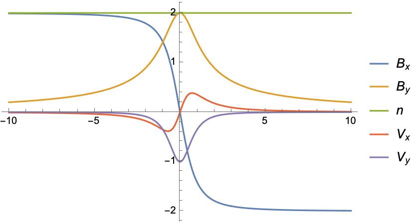
Given \(c = 1/\sqrt{2}\), we have \(B_y \to 0\) as \(z \to \infty\). Profiles are plotted below for \(B_0 = 2\).
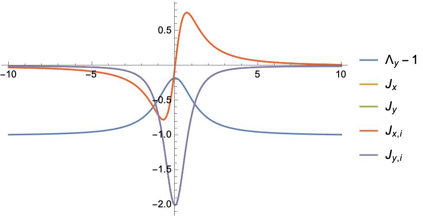
The multi-fluid effect is clearly demonstrated by \(Λ_y - 1\).
Manipulate[
 Block[{B0 = B0i, c = ci},
  p1 = Plot[
    Evaluate[{n[z], Bx[z], By[z], u1x[z], u1y[z]} /. sols //. rulesn],
    {z, -zmax, zmax},
    PlotLegends -> {n, Subscript[B, x], Subscript[B, y], Subscript[u, x], Subscript[u, y]}
  ];
  Export["figures/profiles.jpg", p1];
  p1
  ],

 {{ci, 1/Sqrt[2]}, 0, 2},
 {{B0i, 2}, 0.5, 2},
 {{zmax, 10}, 5, 30}
 ]

Manipulate[
 Block[{B0 = B0i, c = ci, Λz = Λz0},
  p = Plot[
    Evaluate[{Λy - 1, Jxi, Jx, Jyi, Jy} /. sols //.
      rulesn],
    {z, -zmax, zmax},
    PlotLegends -> {Subscript[Λ, y] - 1, Subscript[J,
      x, i], Subscript[J, x], Subscript[J, y, i], Subscript[J, y]},
    PlotRange -> All];
  Export["figures/J_profiles.jpg", p];
  p
  ],

 {{ci, 1/Sqrt[2]}, 0, 2},
 {{B0i, 2}, 0.5, 2},
 {Λz0, 0, 1},
 {{zmax, 10}, 5, 30}
]
For the same asymptotic magnetic field, it is interesting to see how the plasma profiles change with different system parameters.
\[ \text{cond}(n(z), λ_{n,∞}, λ_{z,∞}) = 0 \]
Here we set \(B_y(z=\infty) = 1/2 B_y(z=0)\) and \(B_0 = 2 B_z\), and fix \(λ_{z,∞} = -1\). By varying \(λ_{n,∞}\), we find that the magnetic field profiles are exactly the same, while plasma velocity profiles vary. We normalize the plasma velocity by asympotic Alfvén velocity \(v_{A,∞} = B_0 / \sqrt{n}\), and the profiles are plotted below Figure 1 (b). It could be seen that for \(λ_{n,∞} = 1\), we have zero bulk velocity change across the current sheet in the asymptotic limit.


Different normalization
Normalized the quantities of the ion species
\[ n_α := λ_{αn} n_e \\ u_{αx} := λ_{αu} B_z / \sqrt{n_{e,\infty}} \\ u_{αy} := λ_{αu} B_z / \sqrt{n_{e,\infty}} \\ u_{αz} := λ_{αu} B_z / \sqrt{n_{e,\infty}} \]
\[ θ' = \mp \frac{Λ_u}{B_0} + Γ_e \]
conf = {ratio -> 1/2}
TextString[conf]
<!-- Convert a dict-like configuration to a string -->
saveName[c_] := StringJoin[ToString /@ c]