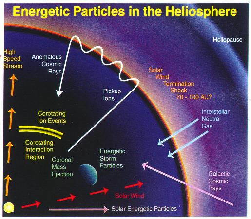
Introduction - Transport of Energetic Particles in the Heliosphere
Desai and Giacalone (2016)
Notes: - Importance of energetic particle transport in astrophysical plasmas.
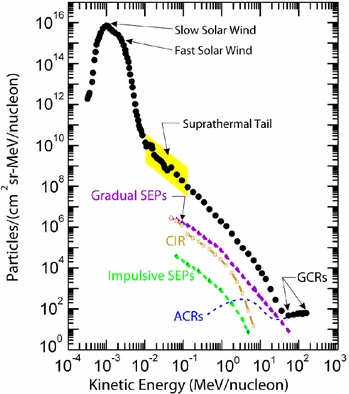
Solar energetic particles, or SEPs, from suprathermal (few keV) up to relativistic (∼few GeV) energies are accelerated near the Sun in at least two ways: (1) by magnetic reconnection-driven processes during solar flares resulting in impulsive SEPs, and (2) at fast coronal-mass-ejection-driven shock waves that produce large gradual SEP events. Large gradual SEP events are of particular interest because the accompanying high-energy (>10s MeV) protons pose serious radiation threats to human explorers living and working beyond low-Earth orbit and to technological assets such as communications and scientific satellites in space. However, a complete understanding of these large SEP events has eluded us primarily because their properties, as observed in Earth orbit, are smeared due to mixing and contributions from many important physical effects.
Introduction - Particle Transport in Turbulent Magnetic Field
Giacalone and Jokipii (1999)
- Parallel diffusion due to pitch-angle diffusion
- Drift motion due to magnetic field inhomogeneities
- Transverse diffusion due to random walk of magnetic lines
Notes: - Role of turbulent magnetic fields in the heliosphere.
Pitch-angle diffusion, connected with transport in the direction parallel to magnetic field, drift motions due to magnetic field inhomogeneities, as well as transverse diffusion due to random walk of magnetic lines are all aspects of energetic particle transport that are controlled by magnetic turbulence properties, such as fluctuation amplitude, spectral index and anisotropy.
Introduction - Turbulence and Coherent Structures
![Cover image: A direct numerical simulation of incompressible magnetohydrodynamic plasma turbulence in the presence of a strong guide field. The resolution of the simulation is 2048x2048x128. The image shows the presence and development of strong current sheets and instabilities in the current density, in one of the planes perpendicular to the guide field. Overlaid on this is an image of a solar prominence eruption observed by the NASA Solar Dynamics Observatory (SDO) on March 16, 2013. Simulation image is provided by Dr. Romain Meyrand and the SDO image is from the SDO Gallery, image 187 [http://sdo.gsfc.nasa.gov/gallery/main/item/187].](https://royalsocietypublishing.org/cms/asset/b9ab350a-66a0-4764-bcbc-d28f1b4f757c/rsta.373.issue-2041.largecover.jpeg)
Hussain (1983)
Notes: - Emphasize that coherent structures have distinct, observable features. - Describe how these structures can dominate scattering processes.
The classical theory of ion scattering is based on consideration of an ensemble of random magnetic field fluctuations [7,8,15], whereas the internal structure of such fluctuations has not been studied in detail.
Introduction - Particle Motion in Magnetic Field
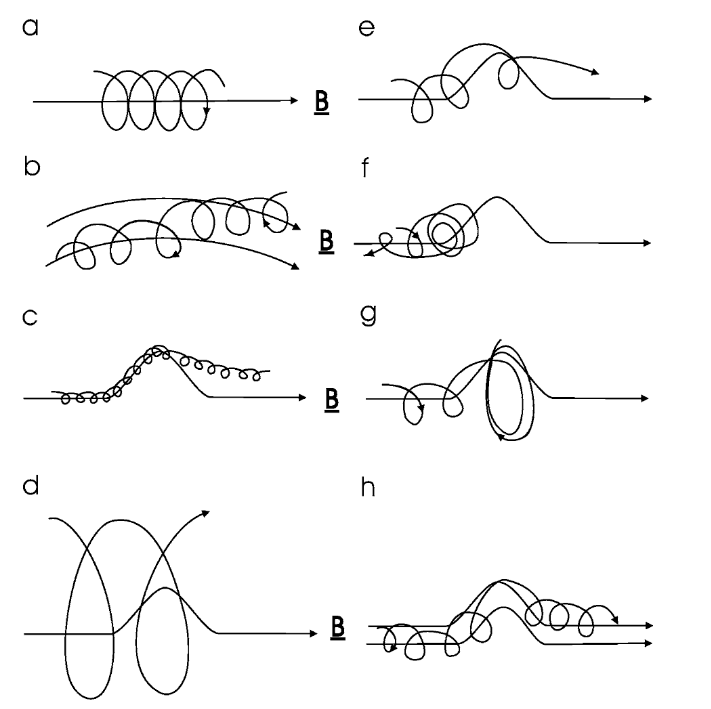
Fig. 1 Charged particle motion in a magnetic field. (a) In a uniform magnetic field the particle has a spiral orbit with a gyroradius rg = P /Bc. (b) When the field is non-uniform the particle drifts away from a field line due to the gradient and curvature of the field. (c) When a particle meets a kink in the field that has a scale length rg , all particles will progress through the kink (but they may drift to adjacent field lines while doing so). (d) Likewise, if rg scale size of the kink, all particles will pass through it without being affected much. (e, f, g) When rg ≈ scale size of the kink, it depends on the gyrophase of the motion when the particles starts to feel the kink whether it will go through the kink (e), be reflected back (f), or effectively get stuck in the kink (g). This process is called pitch-angle scattering along the field. (h) When particles meet such a kink, there is also a scattering in phase angle, which leads to scattering across the field lines, but such that κ⊥ κ‖
Introduction - Current Sheets in the Solar Wind

The Problem: Scattering by Current Sheets
Malara et al. (2023), Malara, Perri, and Zimbardo (2021) Artemyev et al. (2020), Artemyev, Neishtadt, and Zelenyi (2013a), Artemyev, Neishtadt, and Zelenyi (2013b) Zelenyi et al. (2013), Neishtadt (2000) Büchner and Zelenyi (1989), Chen and Palmadesso (1986), Tennyson, Cary, and Escande (1986)
Motivation / Gap : Prior studies lack realistic solar wind statistics &/ large-scale simulation in a realistic magnetic field
How can we quantify the efficiency of ion scattering by solar wind discontinuities?
Image: Schematic of a particle trajectory interacting with a current sheet.
Notes:
- Why current sheets matter: Non-diffusive scattering, chaotic dynamics.
- Gap: Prior studies lack realistic solar wind statistics.
Analytical Model - Magnetic Field Model
\[ \mathbf{B} = B_0 (\cos θ \ \mathbf{e_z} + \sin θ ( \sin φ(z) \ \mathbf{e_x} + \cos φ (z) \ \mathbf{e_y})) \]
\(φ(z) = β \tanh(z/L)\) \(\mathbf{B_z} = B_0 \cos θ \ \mathbf{e_z} \equiv B_n \mathbf{e_z}\) \(\mathbf{B_t} = B_t \sin φ(z) \ \mathbf{e_x} + B_t \cos φ (z) \ \mathbf{e_y}\)
Analytical Model - Hamiltonian Approach
The motion of a particle can be expressed in the Hamiltonian formalism as follows: \[ H = \frac{1}{2m} \left( \mathbf{p} - q \mathbf{A} \right)^2 \]
where \(\mathbf{A}\) represents the magnetic vector potential, \(\mathbf{p}\) is the canonical momentum. More specifically, the magnetic vector potential \(\mathbf{A}\) can be expressed in an exact integrable form:
\[ A_x = L B_t f_1(z),\;\; A_y = L B_t f_2(z) + x B_n, \;\; A_z = 0 \]
- Key Points:
- Introduction to the Hamiltonian formalism in this context.
- Expression for the magnetic vector potential.
- Transition from canonical to dimensionless variables.
- Notes:
- Explain why the Hamiltonian approach is useful for modeling particle dynamics.
- Highlight the derivation steps and the significance of the normalization.
- Image Suggestion:
- Flow diagram summarizing the derivation from the physical Hamiltonian to the dimensionless form.
Analytical Model - Dimensionless Hamiltonian and Asymptotic Expansion
\((x, z) = (\tilde{x} L + c_x, \tilde{z} L)\) and \((p_x, p_z) = p (\tilde{p_x}, \tilde{p_z})\) where \(p = q L B_t/c\) and \(h = q^2 L^2 B_t^2/m c^2\)
\[ \tilde{H} = \frac{1}{2} \left(\left(\tilde{p_x}-f_1(\tilde{z})\right)^2+\left(\tilde{x} \cot θ + f_2(\tilde{z}\right)^2+\tilde{p_z}^2\right) \]
\[ f_1 (\tilde{z}) =\frac{1}{2} \cos β \ \left(\text{Ci}\left(βs_+(\tilde{z}) \right)-\text{Ci}\left(βs_-(\tilde{z})\right)\right) + \frac{1}{2} \sin β \ \left(\text{Si}\left(βs_+(\tilde{z}) \right)-\text{Si}\left(βs_-(\tilde{z})\right)\right), \] \[ f_2 (\tilde{z}) =\frac{1}{2} \sin β \ \left(\text{Ci}\left(β s_+(\tilde{z}) \right)+\text{Ci}\left(β s_-(\tilde{z})\right)\right) -\frac{1}{2} \cos β \ \left(\text{Si}\left(β s_+(\tilde{z}) \right)+\text{Si}\left(β s_-(\tilde{z})\right)\right) \]
\[ f_1 (z) ~ z - \frac{1}{6} \beta ^2 z^3 + O\left(z^4\right) \] \[ f_2 (z) ~ \frac{\beta z^2}{2} + O\left(z^4\right) \]
Adiabatic Invariance and Pitch Angle
Variables \((κ x, p_x)\) change much slower than \((z, p_z)\) (for κ << 1),
Generalized magnetic moment \(I_z = (2 π)^{-1} ∮ p_z dz\) is conserved as the first adiabatic invariant with exponential accuracy
Simultaneous conservation of energy and \(I_z\) fully determines the motion of the particle \(\mathbf{v} = \mathbf{v}(\mathbf{r}, I_z, H)\)
In the absence of \(I_z\) destruction, there is no pitch-angle scattering
- Key Points:
- Definition of adiabatic invariance and the magnetic moment (I_z).
- Conditions under which the adiabatic invariant is conserved.
- Notes:
- Explain the concept of adiabatic invariance in simple terms.
- Discuss why maintaining (I_z) is important for particle trajectory predictions.
- Image Suggestion:
- Diagram depicting adiabatic invariance with trajectories in phase space.
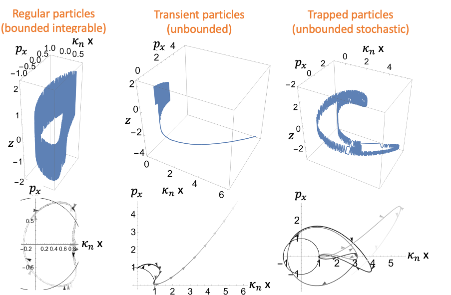
Destruction of Adiabatic Invariance: Separatrix and Uncertainty Curve
- Two distinct types of particle trajectories in \((z, p_z)\) plane separated by a curve called Separatrix.
- The separatrix corresponds to a point on a certain curve in the \((κ x, p_x)\) plane, called Uncertainty Curve.
Near the separatrix, the instantaneous period of motion increases logarithmically. Particle accumulates a nonvanishing change in the adiabatic invariant.
- Dynamical jump
- Geometric jump
Uncertainty curve
The length of uncertainty curve, \(L_{\text{uc}}/\sqrt{H}\), is a good estimate of a phase space volume filled by trajectories experiencing strong scattering. This length increases with \(β\) (for fixed \(H\)) and with \(H\) (for fixed \(β\)). Thus, the scattering probability is higher for larger magnetic field rotation angles and for large particle energy.

Part 2
In the first part, we introduced the basic physics of ion scattering by the solar wind.
Takeaway 1: Larger magnetic field rotation angles and higher particle energies lead to larger chance of pitch-angle scattering.
In the following part, we will focus on the test particle simulations to quantify the ion scattering by the solar wind current sheets.
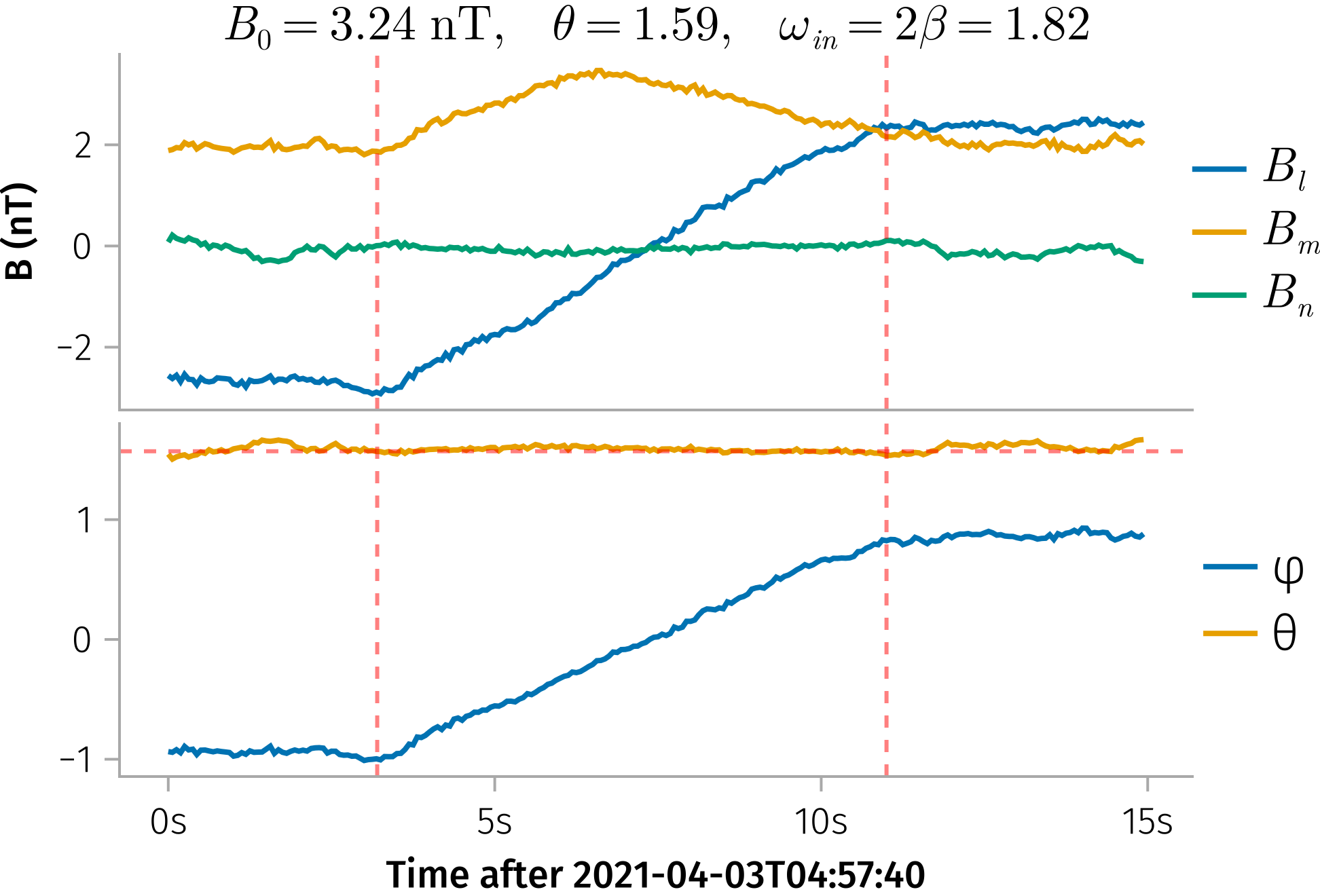
Test Particle Simulations - Solar Wind Current Sheet Dataset
\(Δ|B|/|B| > 0.05\) or \(ω > 60°\) (Liu et al. 2023)
The most probable values in the 3D distribution are a characteristic velocity (\(v_0\)) of approximately 250 km/s, a in-plane rotation angle (\(ω_{in}\)) about 90 degrees, and an azimuthal angle (\(θ\)) of around 85 degrees.
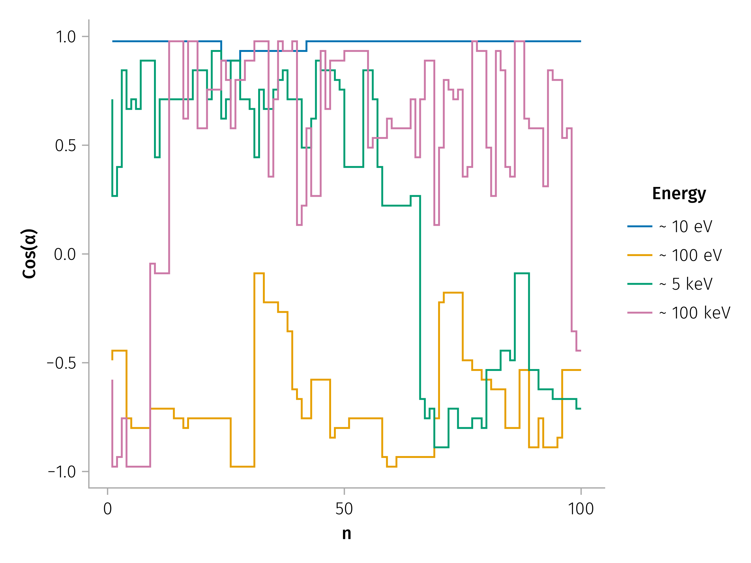
Examples of Pitch Angle Scattering
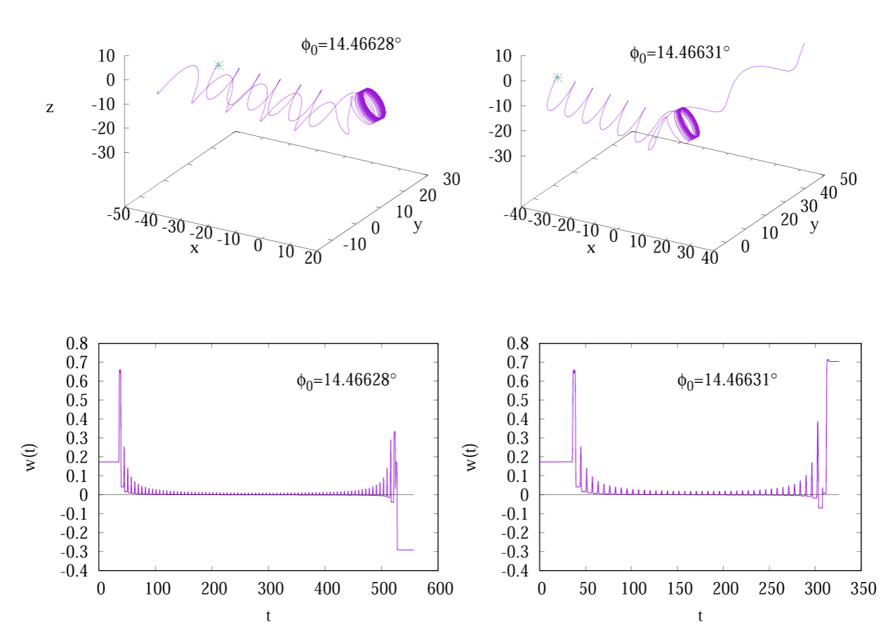
” Motion of particles crossing the discontinuity is extremely complex and highly sensitive to the initial conditions of the system, with transitions to a chaotic behavior. Malara, Perri, and Zimbardo (2021) ”
\(\cos α\)
Scattering process \(\Pi : (α_0, ψ_0) \to (α_1, ψ_1)\) is better represented as a probabilistic transition \(p(α_1 | α_0, \Pi)\)
Transition Matrix
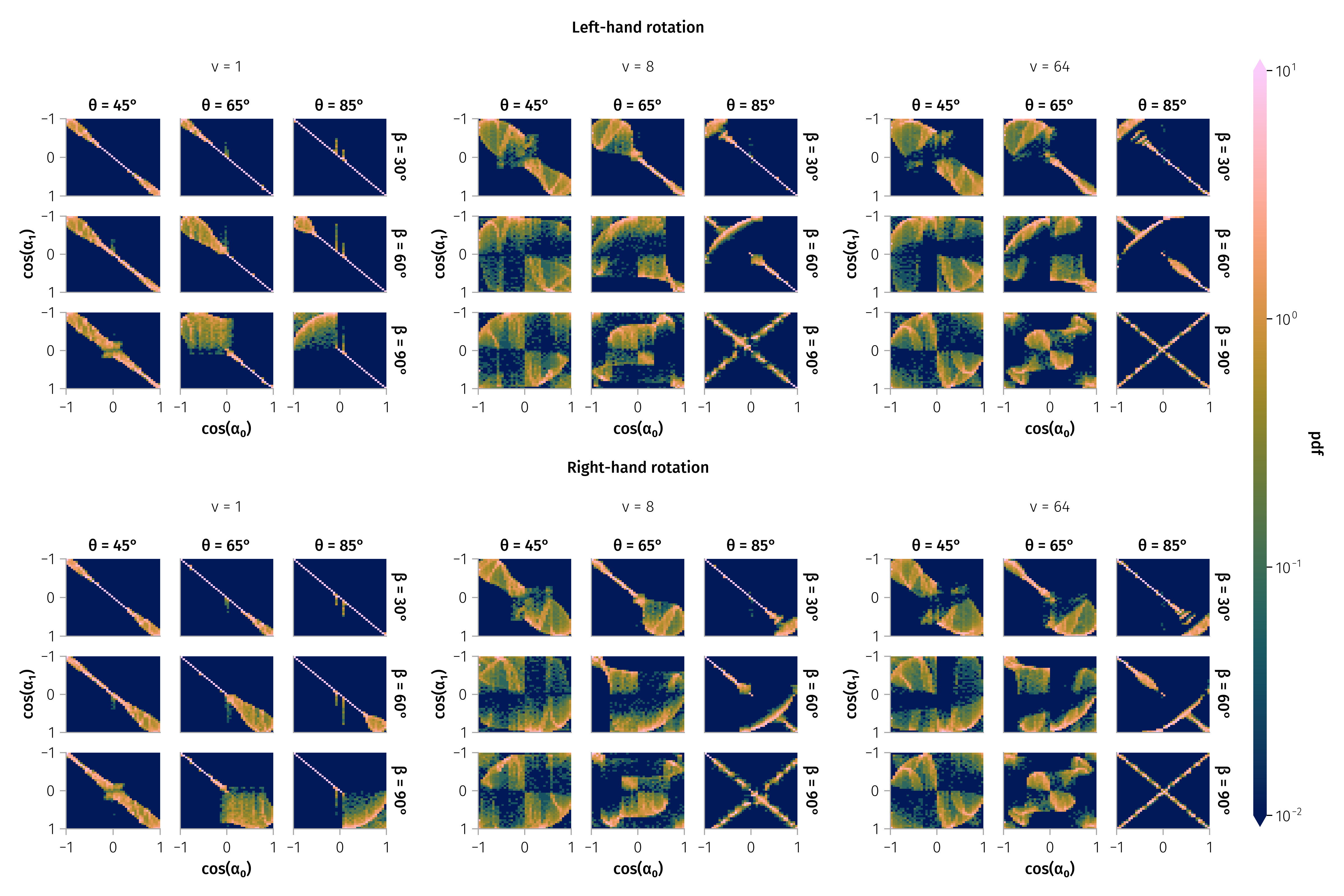
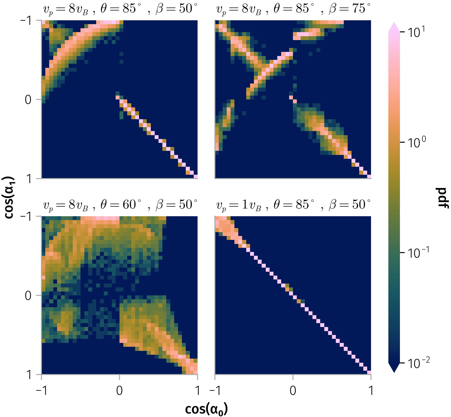
Pitch angle scattering by typical discontinuity
With in-plane rotation angle (\(ω_{in}\)) about 90 degrees, and azimuthal angle (\(θ\)) of around 85 degrees. Luckily, higher or lower energy do not exhibit apparently different scattering probabilities.
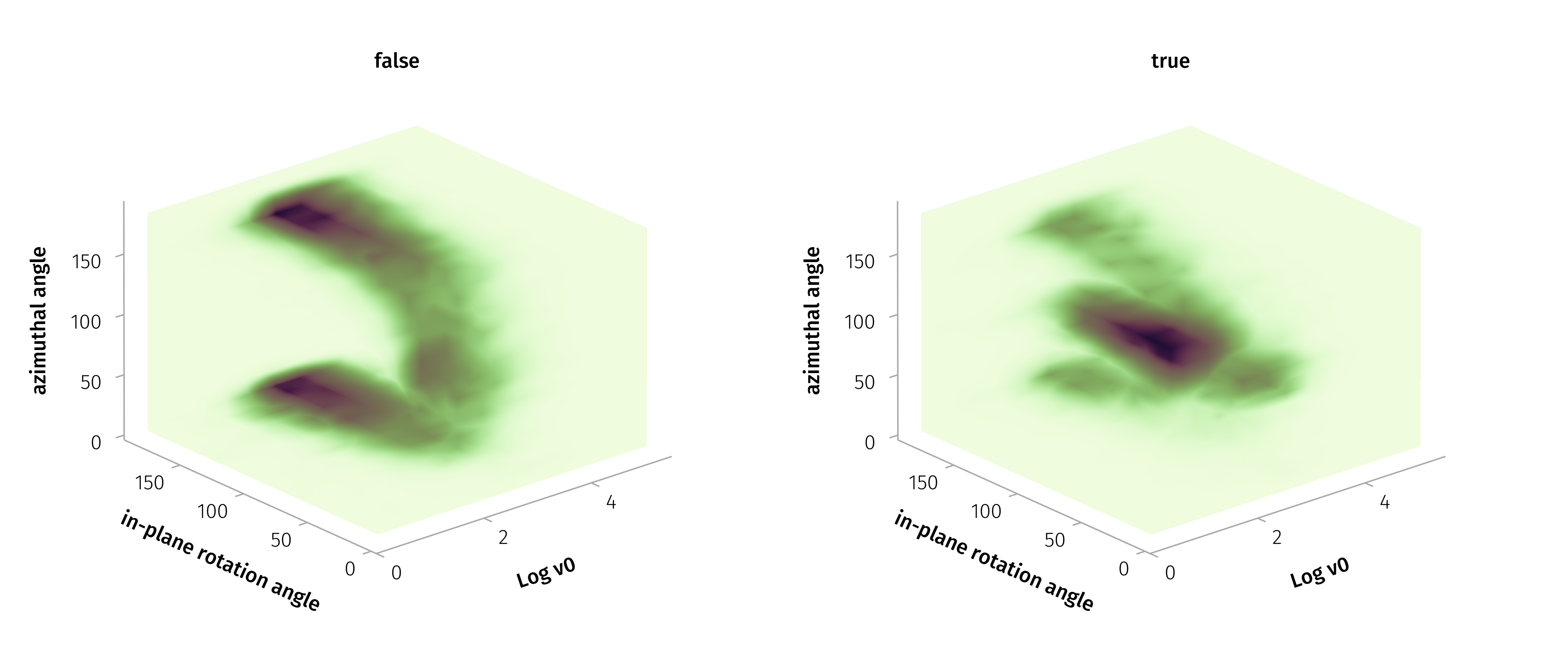
Weighted Transition Matrix
Aggregates scattering probabilities across observed current sheets. \(p(α_1 | α_0, \Pi)\) => \(p(α_1 | α_0) = \sum_{i} p(α_1 | α_0, \Pi_i) w_i\)
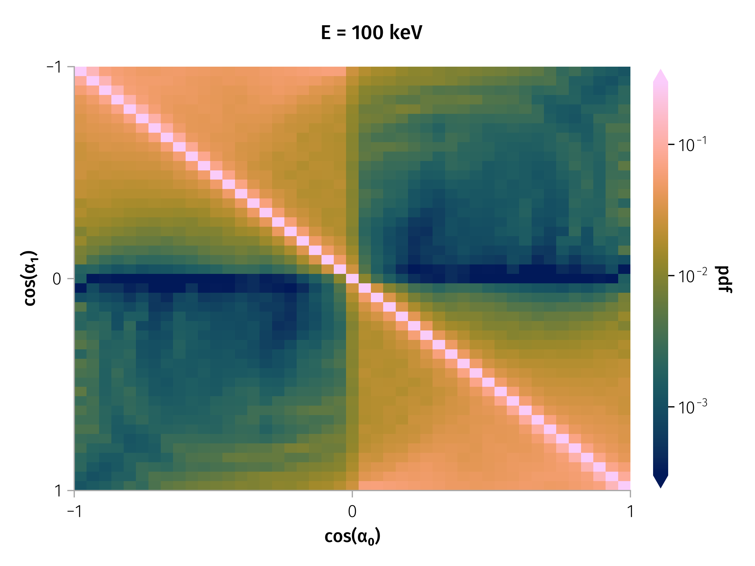
Image: WTM heatmap from fig-tm-stats-100keV.
Notes:
- Aggregates scattering probabilities across observed current sheets.
- Bright diagonal = most particles weakly scattered.
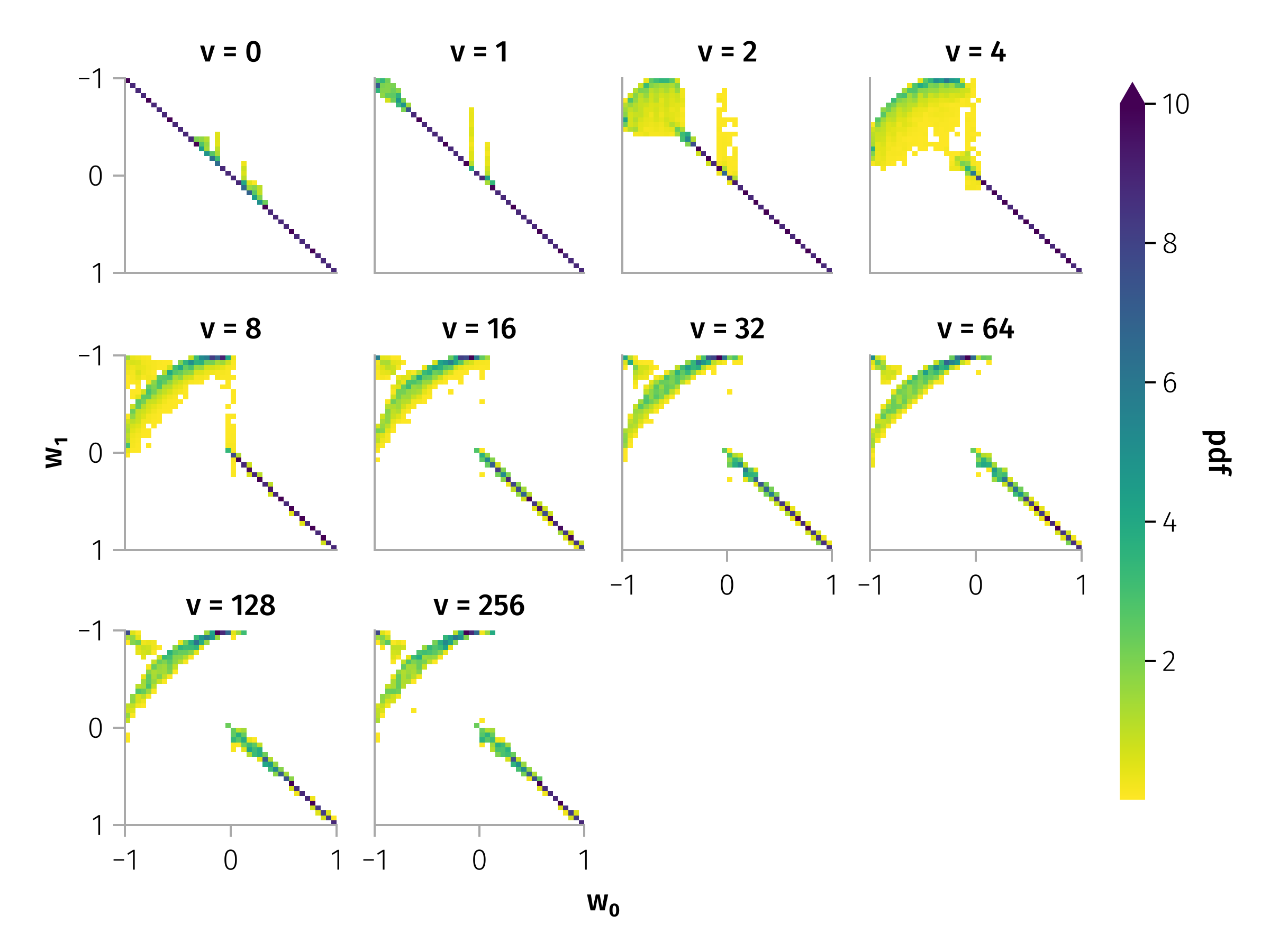
Long-Term Pitch Angle Evolution
\[α_{n+1,i} = W\left(α_{n,i}, ξ_{n,i}\right)\]
Notes:
- Rare large-angle jumps drive rapid mixing.
Scattering Rate Coefficients
\[ \begin{aligned} M_1(n) = N^{-1}∑_{i=1}^N (α_{n,i} - α_{0,i}) \\ M_2(n) = N^{-1}∑_{i=1}^N (α_{n,i} - α_{0,i})^2 - M_1^2(n) \end{aligned} \]
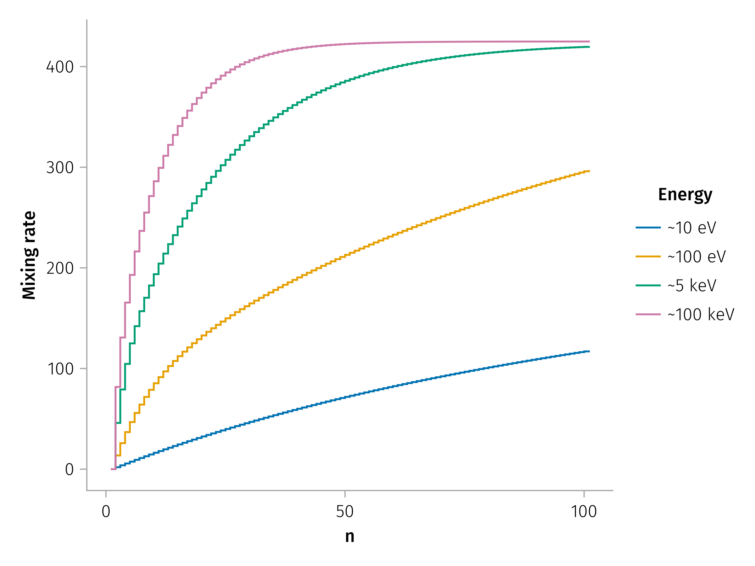
Pitch angle scattering => Parallel Diffusion

- Notes:
- (D_{nn}) quantifies scattering efficiency.
- (D_{nn}) quantifies scattering efficiency.
Implications for Particle Transport
\(h = \frac{q^2 L^2 B_t^2}{m c^2}\)
\(B \sim 1/r\) and \(L \sim d_i ~ n^{-1/2} ~ r\) => continuous scattering by current sheets during propagation => higher occurrence rate of current sheets closer to the Sun => ???Large gradual solar energetic particle events???
- Key Points:
- Impact on spatial diffusion and acceleration processes.
- Connection between enhanced pitch-angle scattering and reduced acceleration timescales in shocks.
- Broader relevance for heliospheric and astrophysical plasma transport.
- Notes:
- Summarize how the research improves our understanding of energetic particle dynamics.
- Emphasize the potential integration of these results into global transport models.
- Image Suggestion:
- Conceptual diagram linking pitch-angle scattering, spatial diffusion, and particle acceleration in shock environments.
Conclusions, Future Work & Q&A
- Key Points:
- Recap of major findings: analytical model, simulation results, and effective scattering rate.
- Future directions: investigation of cross-field diffusion, model refinement, and further observational studies.
- Notes:
- Summarize the key contributions of the research.
- Invite audience questions and provide contact information for follow-up discussions.
- Image Suggestion:
- A summary graphic or montage that visually encapsulates the research process and findings, with space for contact details.