
| Mission | \(\delta t_B\) | \(\delta t_{plasma}\) | Radial coverage | Launch date | website |
|---|---|---|---|---|---|
| Juno | 1 Hz | 1 - 5.5 AU | 2011-08-05 00:00:00 | [‘NASA’] | |
| ARTEMIS | 5 Hz, … | 2007-02-17 00:00:00 | |||
| STEREO-A | 8 Hz | 2006-10-26 00:00:00 | |||
| WIND | 11 Hz | 1994-11-01 00:00:00 | [‘NASA’] | ||
| Solar Orbiter | 0.28 - 0.9 AU | 2020-02-10 00:00:00 | [‘ESA’] | ||
| Parker Solar Probe | 0.05 - 1 AU | 2018-08-12 00:00:00 | [‘NASA’] |
Plain Language Summary
What I did: I studied the solar wind discontinuities in the outer heliosphere using data from the Juno spacecraft during its cruise phase. I identified and analyzed the properties of the discontinuities at different radial distances from the Sun. I differentiated the temporal effect (correlated with solar activity) and spatial variations (correlated with radial distance).
What I found: The normalized occurrence rate of IDs drops with the radial distance from the Sun, following a \(1/r\) law. The thickness of IDs increases with the radial distance from the Sun, but after normalization to the ion inertial length, the thickness of IDs decreases. The current intensity of IDs decreases with the radial distance from the Sun, but after normalization to the Alfven current, the current intensity of IDs increases.
What it means: The results of this study provide a better understanding of the solar wind discontinuities in the outer heliosphere and their spatial evolution. This information is important for understanding the dynamics of the solar wind and testing the local generation mechanism of discontinuities.
Introduction
Rapid variations in interplanetary magnetic fields, commonly recognized as solar wind magnetic discontinuities (Colburn and Sonett 1966), embody localized transient rotations or jumps of the magnetic field. Considered important for efficient plasma heating, they carry the most intense currents found in the solar wind and obserrved throughout the heliosphere from inner heliosphere (Liu, Fu, Cao, Yu, et al. 2022) to the heliosheath (Burlaga and Ness 2011). Theoretical models (Lerche 1975; Medvedev et al. 1997) and MHD simulations (Greco et al. 2008, 2009; Yang et al. 2015) suggest that the formation and destruction of discontinuities are closely related to the nonlinear dynamics of Alfvén waves and/or Alfvénic turbuluence. These nonlinear processes can create significant isolated disturbances to the otherwise adiabatic evolution of the solar wind flow (?Reference?) and host many processes, including magnetic reconnection (?Reference?) and Fermi acceleration of particles (Wentzel 1964). Moreover, they contribute significantly to the magnetic fluctuation spectra (Borovsky 2010) and can affect space weather (Tsurutani et al. 2011). Therefore, the study of the spatial evolution of solar wind discontinuities is important for understanding the dynamics of the solar wind and test the local generation mechanism of discontinuities. However, previous study of solar wind discontinuities evolution (Söding et al. 2001) in the outer heliosphere were rarely in conjunction with measurements closer to the Sun. Moreover, the intervals in their study spread over multiple solar cycles though they are selected during solar activity minimum. Thus it is presently unclear whether their frequency and properties are the result of solar variability or due to the natural evolution of the discontinuities during their propagation and interaction with the ambient solar wind.
The goal of our paper is to investigate, statistically, discontinuities at different radial distance in the outer heliosphere to obtain a understanding of their formation and evolution. Our methodology involves integrating Juno measurements (Connerney et al. 2017) between \(1\) and \(5\) AU with those at \(1\) AU to distinguish temporal effect and spatial variations by examining the discontinuity characteristics at two radial distances simultaneously.
First, the missions, instruments and data used are listed. Then, we briefly describe the method used to identify the discontinuities and the model used to estimate the plasma state at Juno location due to the lack of plasma data during its cruise phase. Finally, we present the results of the spatial evolution of the discontinuities with respect to their characteristics (spatial scales and current density), and discuss the implications of our findings.
Dataset, models, and methods
Dataset
In this study we use datasets of four missions measuring solar wind magnetic field and plasma. Synergistic observations of these missions should advance our understanding of the solar wind discontinuities, their radial distribution and evolution (Velli et al. 2020).
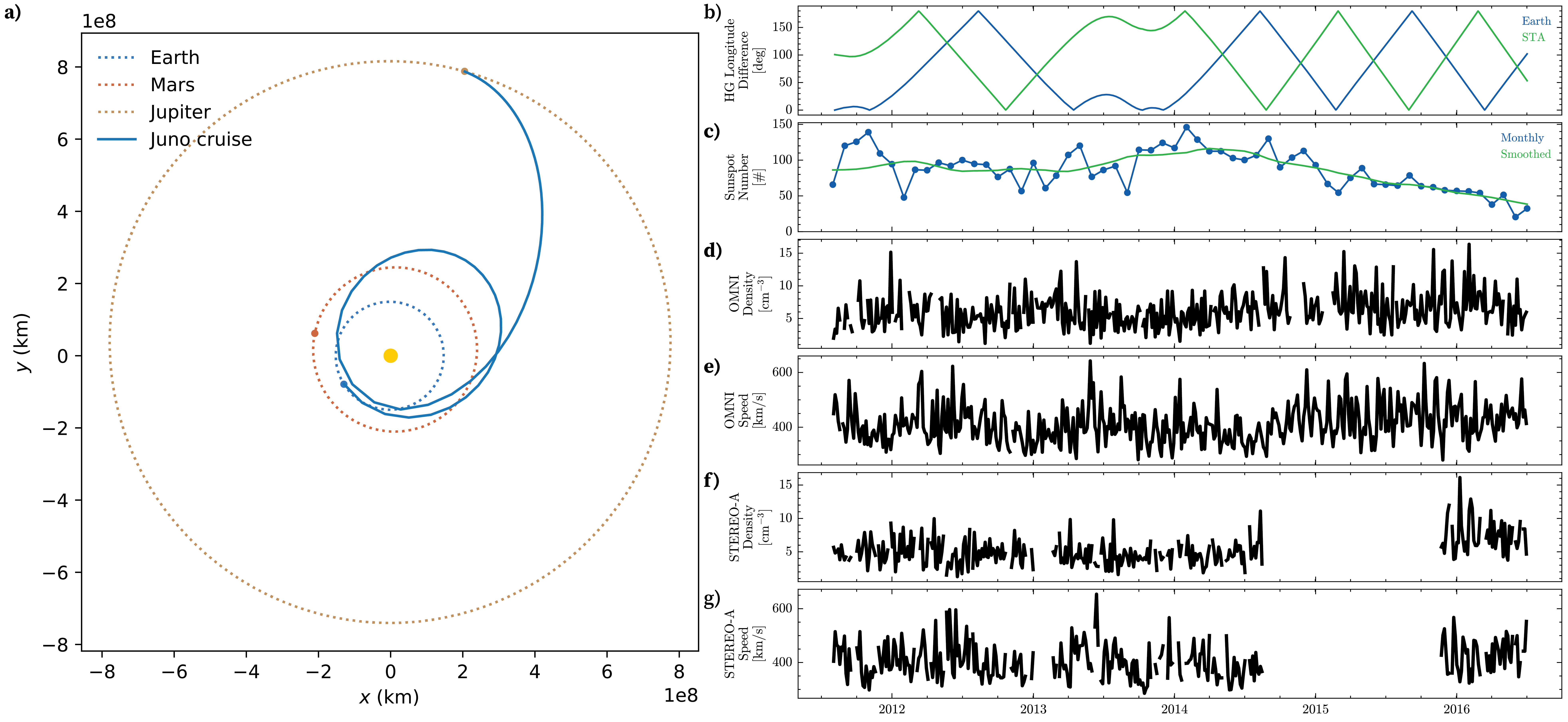
The solar wind plasma state, as evidenced by the sunspot number (referenced in Figure 1), plays a crucial role in understanding the dynamics of discontinuities. During the initial phase of the JUNO mission, the sunspot number reached its peak, indicating a period of heightened solar activity. However, by the end of the mission’s cruise phase, there was a significant decline in solar activity. This variation underscores the importance of calibrating the discontinuity properties in relation to solar activity levels to account for temporal fluctuations.
Furthermore, an analysis of Figure 1 reveals the significance of the heliographic longitudinal difference between the Juno mission and Near-Earth missions (such as Wind and ARTEMIS) as well as STEREO-A missions. This longitudinal discrepancy ensures comprehensive coverage of the plasma en route to Juno. Specifically, when there is a substantial longitudinal difference between Juno and Earth, the difference between Juno and STEREO-A tends to be minimal, and vice versa. This relationship facilitates an extensive observation network for the plasma traveling towards Juno.
The time resolution of the magnetic field and plasma data for Juno, Wind, ARTEMIS, STEREO is summarized in the table below.
Model
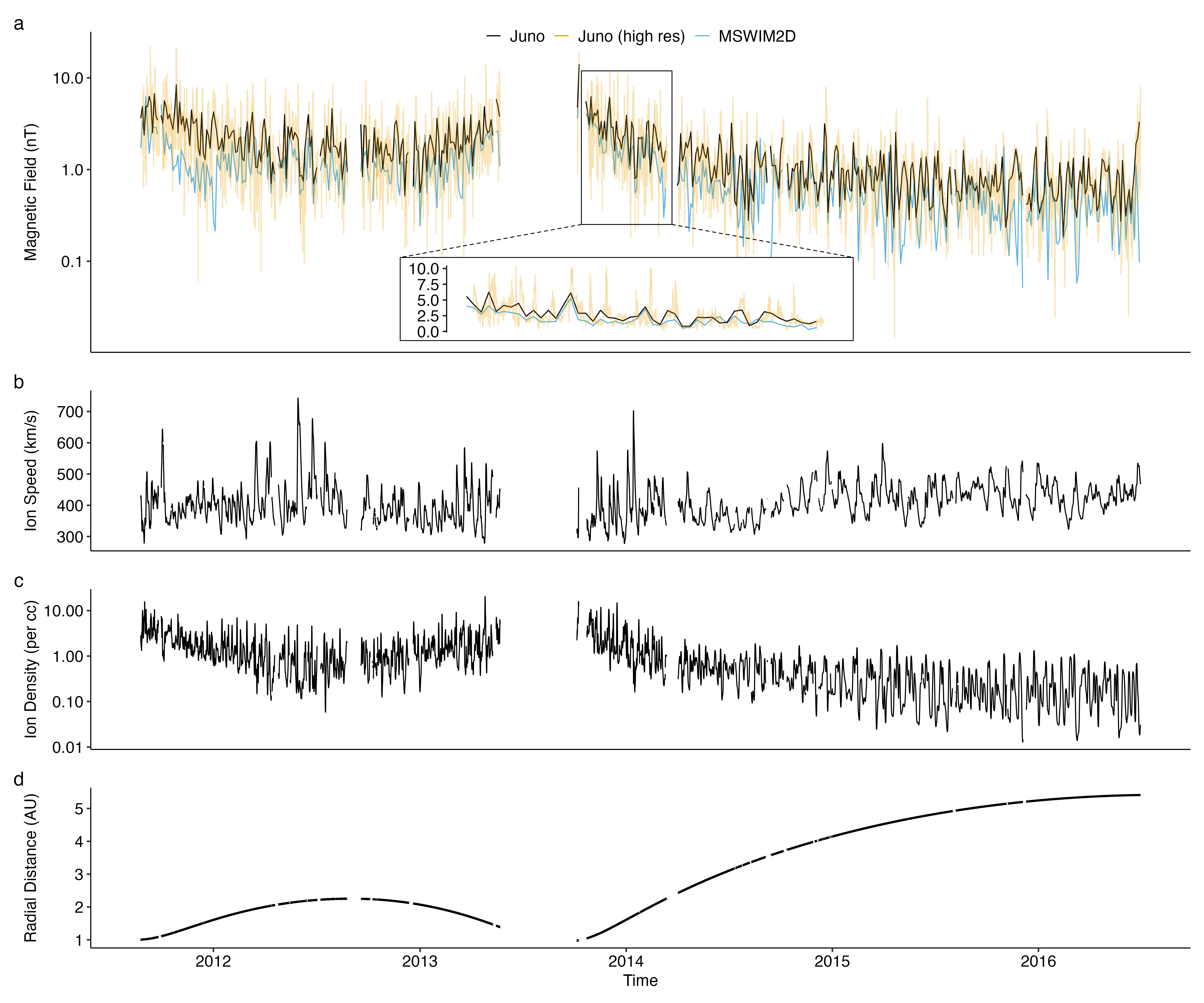
June measurements do not include plasma characteristics, and to estimate discontinuity spatial scale (thicknesses) we will use solar wind speed obtained from the model of solar wind propagation. The hourly solar wind model data from the Two-Dimensional Outer Heliosphere Solar Wind Modeling (MSWIM2D) (Keebler et al. 2022) will be employed to determine the ion bulk velocity \(v\) and plasma density \(n\) at the location of the Juno mission. Utilizing the BATSRUS MHD solver, this model is capable of simulating the propagation of the solar wind from 1 to 75 astronomical units (AU) in the ecliptic plane, effectively encompassing the region of interest for our study. Figure 2 shows comparison of magnetic field magnitudes obtained from MSWIM2D and measured by Juno.
The model time resolution is hourly. After averaging Juno data to the same time resolution, we see that the model data is consistent with the Juno magnetic field data.
Methods
We use Liu’s (Liu, Fu, Cao, Wang, et al. 2022) method to identify discontinuities in the solar wind. This method has better compatibility for the discontinuities with minor field changes, and is more robust to the situation encountered in the outer heliosphere. For each sampling instant \(t\), we define three intervals: the pre-interval \([-1,-1/2]\cdot T+t\), the middle interval \([-1/,1/2]\cdot T+t\), and the post-interval \([1/2,1]\cdot T+t\), in which \(T\) are time lags. Let time series of the magnetic field data in these three intervals are labeled \({\mathbf B}_-\), \({\mathbf B}_0\), \({\mathbf B}_+\), respectively. Then for an discontinuity, the following three conditions should be satisfied: (1) \(\sigma({\mathbf B}_0) > 2\max\left(\sigma({\mathbf B}_-), \sigma({\mathbf B}_+)\right)\), (2) \(\sigma\left({\mathbf B}_-+{\mathbf B}_+\right)>\sigma({\mathbf B}_-)+\sigma({\mathbf B}_+)\), and (3) \(|\Delta {\mathbf B}|>|{\mathbf B}_{bg}|/10\), in which \(\sigma\) and \({\mathbf B}_{bg}\) represent the standard deviation and the background magnetic field magnitude, and \(\Delta {\mathbf B}={\mathbf B}(t+T/2)-{\mathbf B}(t-T/2)\). The first two conditions guarantee that the field changes of the discontinuity identified are large enough to be distinguished from the stochastic fluctuations or Alfven waves on magnetic fields, while the third is a supplementary condition to reduce the uncertainty of recognition.
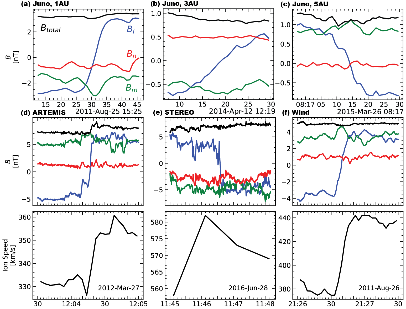
Then for each discontinuity identified, we calculate the distance matrix of the time series sequence (distance between each pair of magnetic field vectors) to determine the leading edge and trailing edge of the discontinuity. After that, we use the minimum or maximum variance analysis (MVA) analysis (Bengt U. Ö. Sonnerup and Scheible 1998; B. U. Ö. Sonnerup and Cahill Jr. 1967) to get the main (most varying) magnetic field component, \(B_l\), and medium variation component, \(B_m\). The maxium variance direction is then fitted by a step-like functions to extract the parameters to properly describe the discontinuity (we used logistic function here). Then we combine the magnetic field data and plasma data to obtain the thickness and the current density of the discontinuity.
\[ B(t; A, \mu, \sigma, {\mathrm{form=logistic}}) = A \left[1 - \frac{1}{1 + e^{\alpha}} \right] \]
where \(\alpha = (t - \mu)/{\sigma}\).
Figure 3 shows several examples of solar wind discontinuities detected by different spacecraft.
Results
Occurrence rate
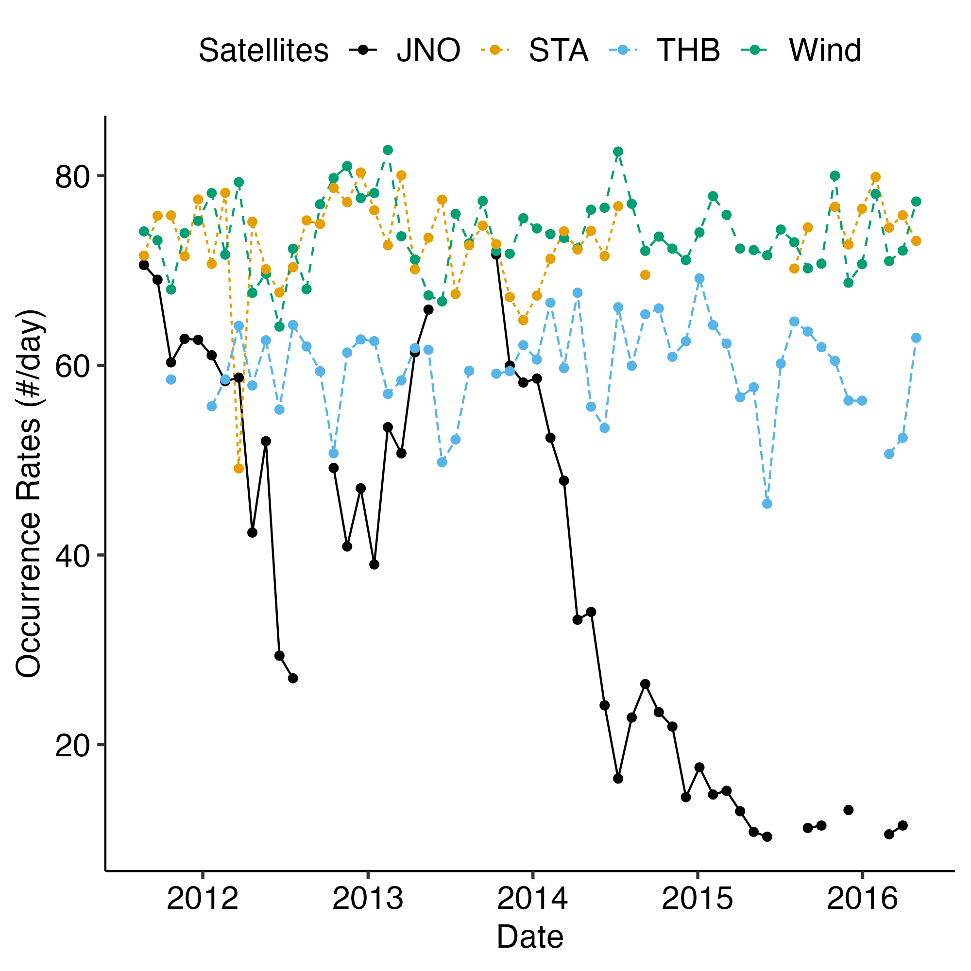
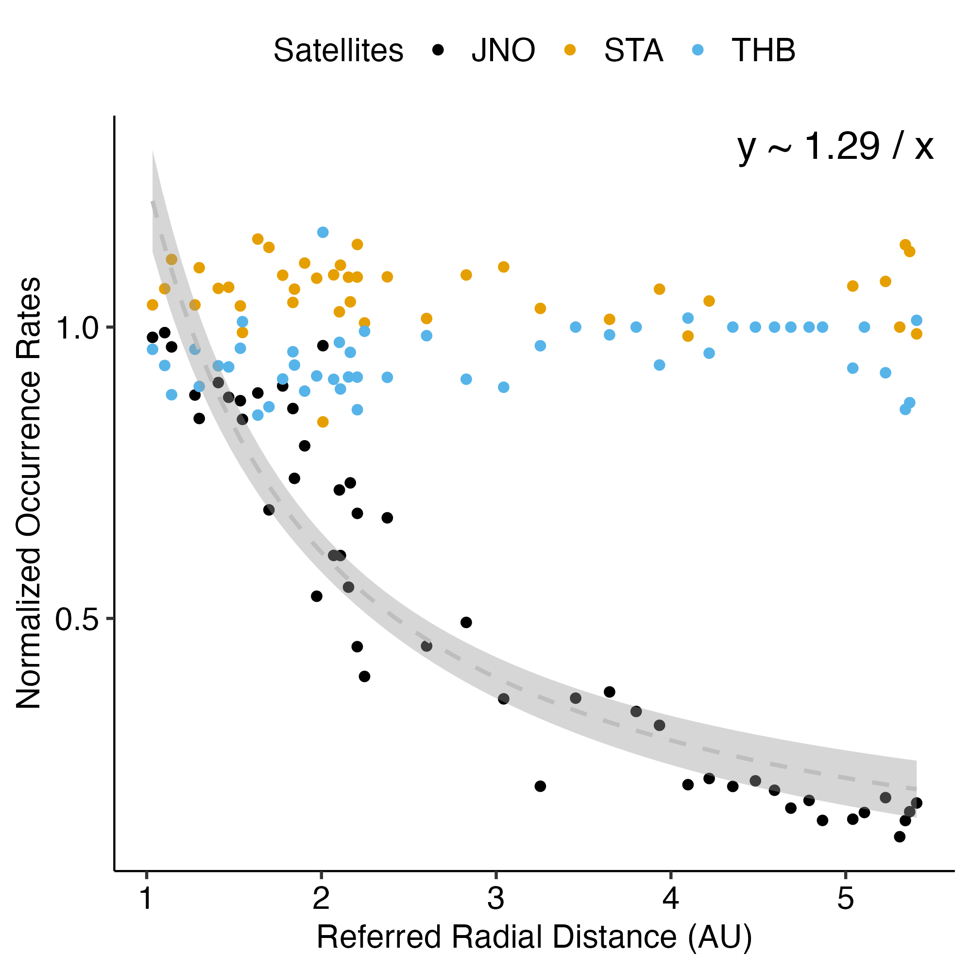
The occurrence rate of IDs is investigated with regards of the radial distance from the Sun.
Note the quantity of IDs per day is corrected with respect to data gap and the time the mission spent in the pristine solar wind. ARTEMIS spacecrafts will only be exposed in the solar wind for a relative short time during its orbits around the Moon and the Moon would be in the magnetosphere for a long time as it orbits the earth. (The data is obtained from OMNIWEB, link: omniweb.gsfc.nasa.gov/ftpbrowser/themis_b_sw.txt)
The rate of occurrence depends linearly on the solar wind velocity (Söding et al. 2001), however the plasma velocity data in Juno mission is not available during its cruise phase. Therefore, we do not normalize the occurrence rate with respect to the solar wind speed. This influence of the solar wind speed on the occurrence rate might be mitigated by the fact all the spacecrafts are in the ecliptic plane, and the solar wind speed is not expected to change significantly with the radial distance from the Sun beyond \(1\) AU. So the decrease of the occurrence rate with the radial distance from the Sun is expected to be a real effect of the radial distance from the Sun.
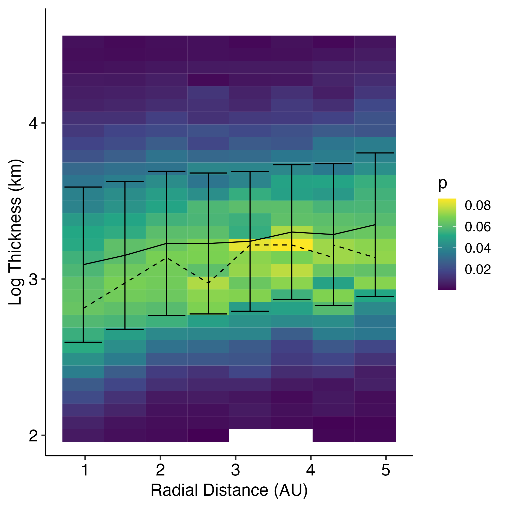
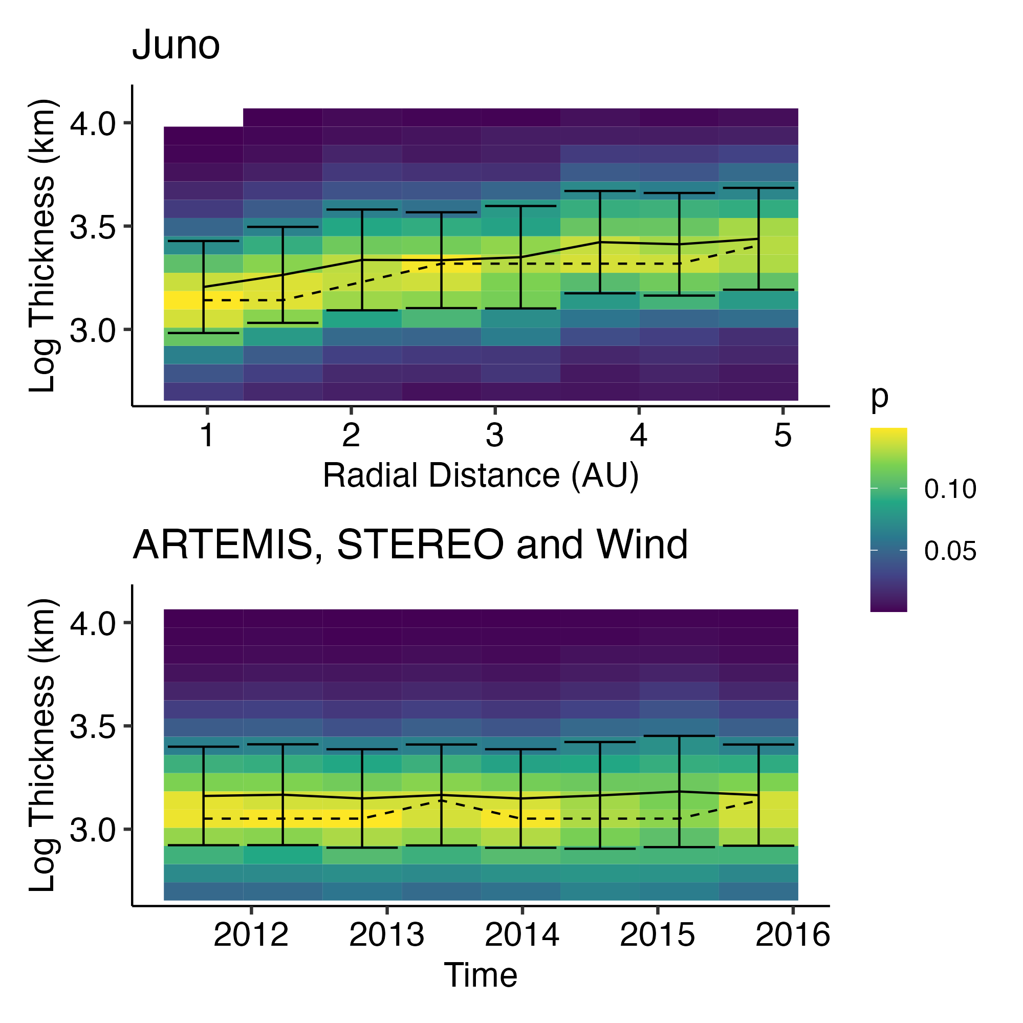
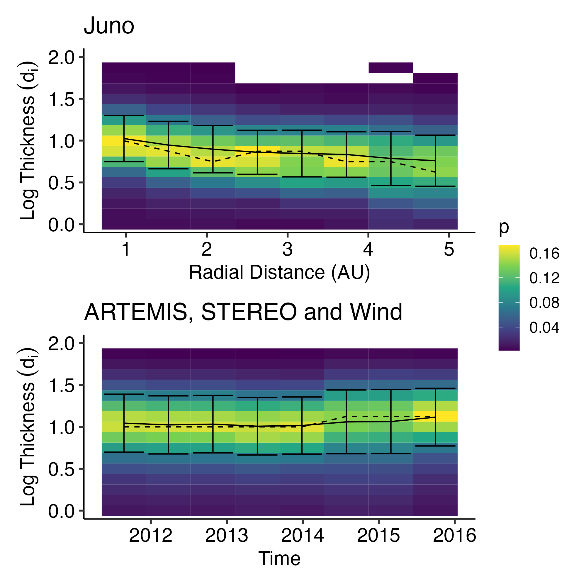
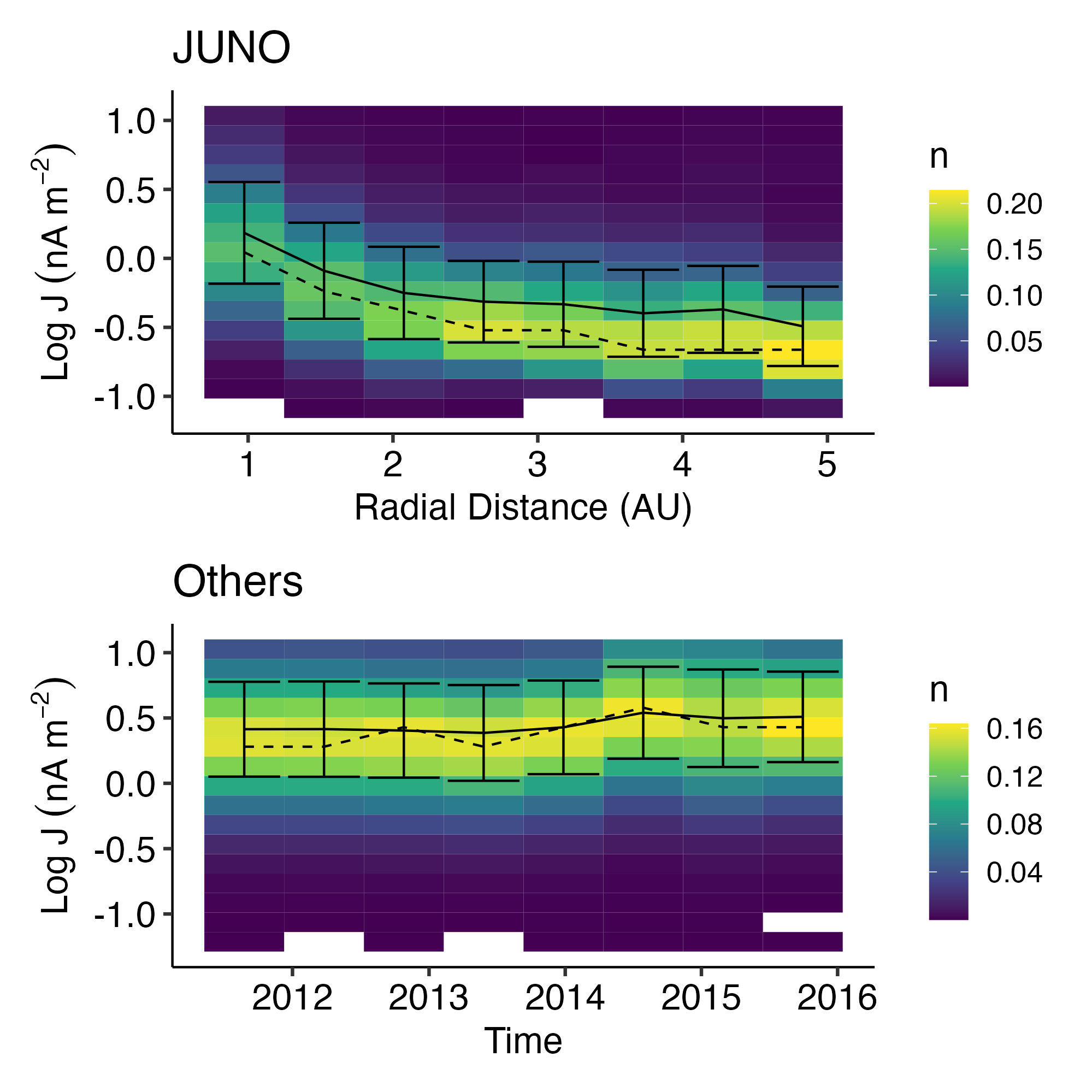
Thickness
The thickness \(d\) of a discontinuity is determined by
\[ d = (v \cdot n) \Delta T \]
with \(v = v_{sw} - v_{s/c} + U\) , where \(\Delta T\) is the transition time (a factor of the \(sigma\) used in fitting) , \(v_{sw}\) is the solar wind velocity. The velocity of the spacecraft \(v_{s/c}\) and the propagation speed of the discontinuities \(U\) are negligible in our case.
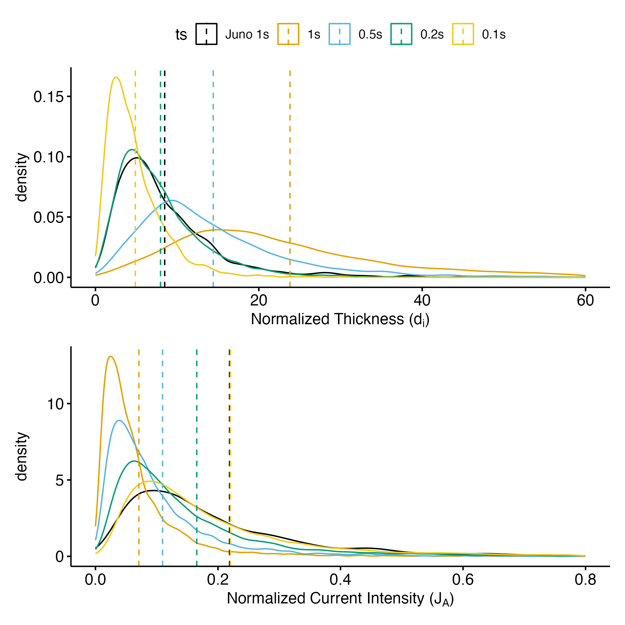
The transition time \(\Delta T\) is determined in one second resolution data for all our missions to reduce the system error. (Note that highest time resolution of the data is not needed for the transition time determination by fitting method, see discussion in the appendix).
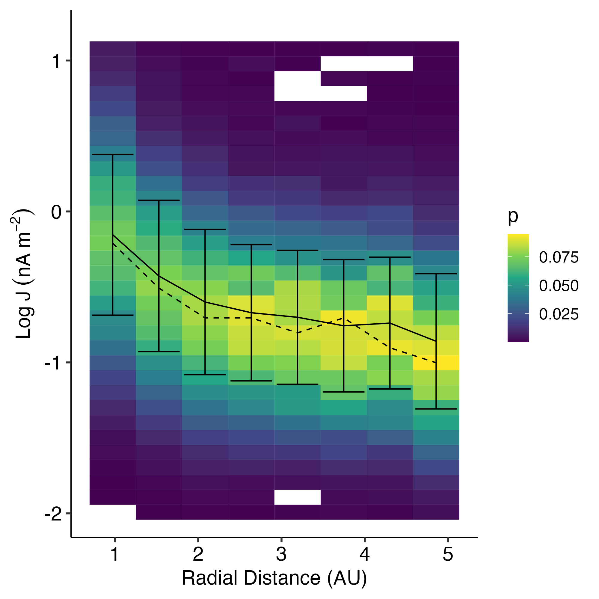
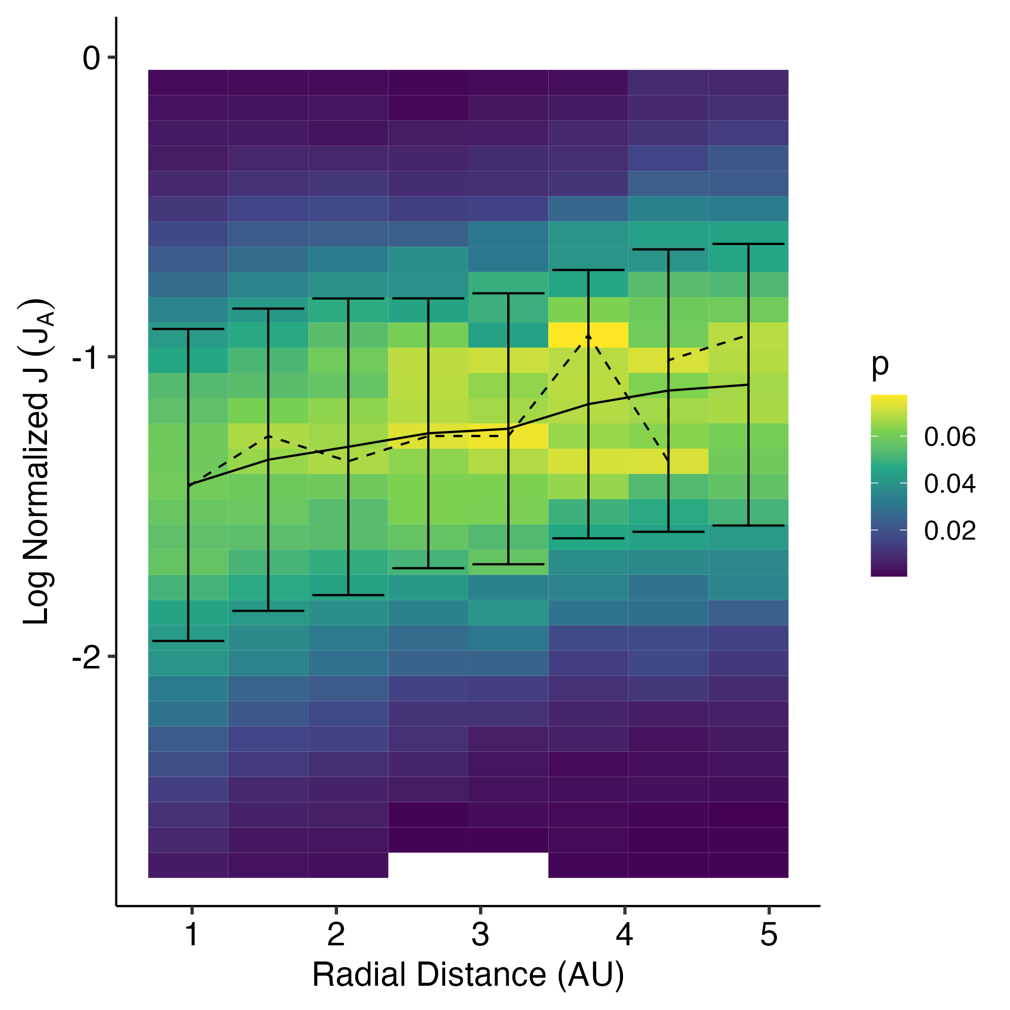
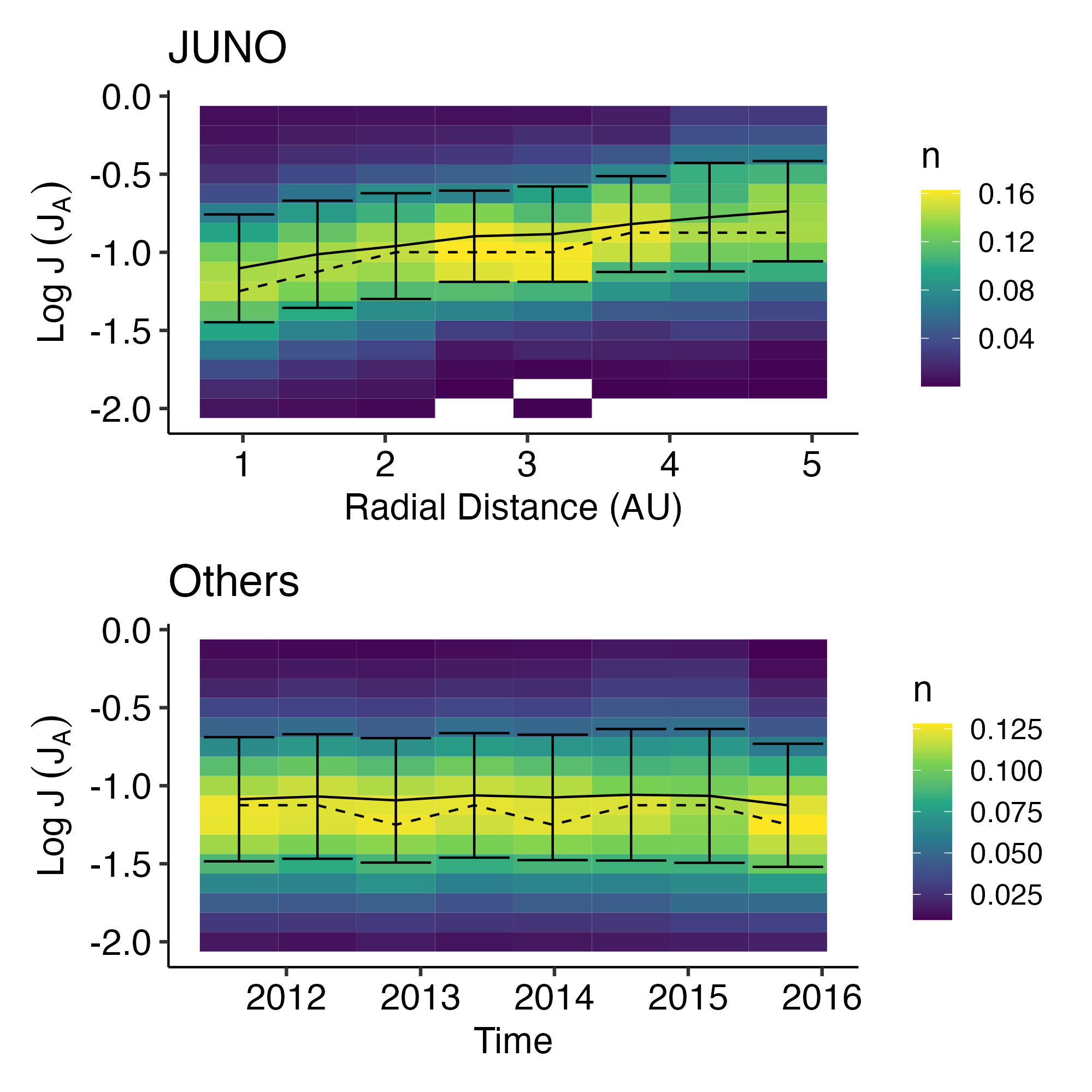
Current density
The peak current density \(J_m\) of a discontinuity is determined by
\[ J_m = - \frac{1}{\mu_0 V_n} \frac{d B_m}{d t}, \]
where \(\mu_0\) is the vacuum permeability and \(V_n\) is the normal component of the proton flow velocity.
Summary and discussion
We have collected 5 years of solar wind discontinuities from JUNO, ARTEMIS and STEREO.
Occurrence rate
The normalized occurrence rate of IDs drops with the radial distance from the Sun, following \(1/r\) law.
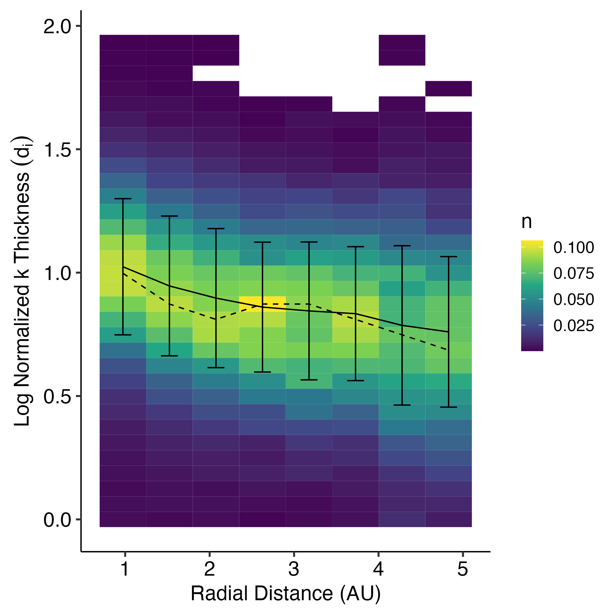
Thickness
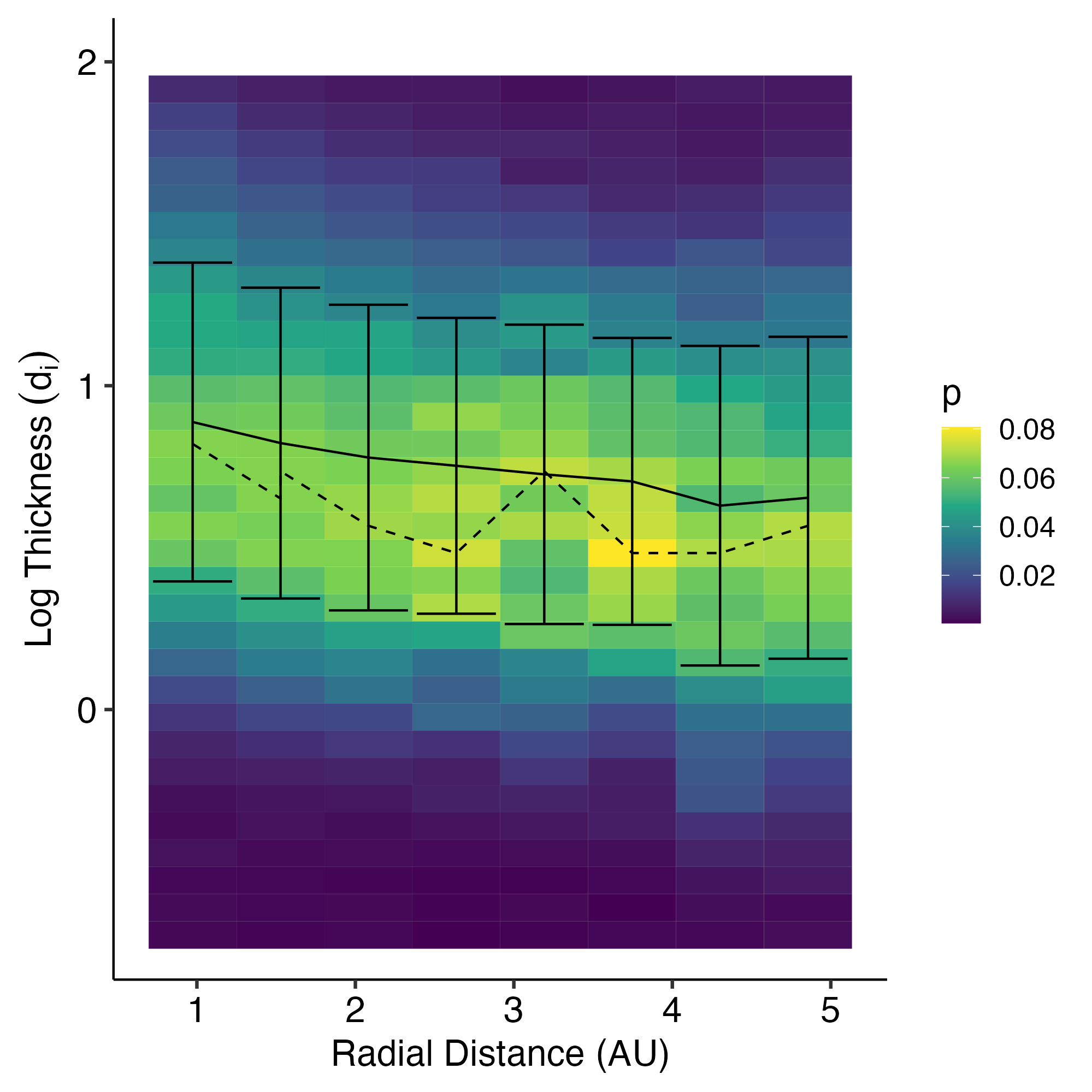
The thickness of IDs increases with the radial distance from the Sun, but after normalization to ion inertial length, the thickness of IDs decreases.
Current density
The current density of IDs decrease with the radial distance from the Sun, but after normalization to the Alfven current , the current density of IDs increases.
Acknowledgements
Sunspot data from the World Data Center SILSO, Royal Observatory of Belgium, Brussels. ARTEMIS solar wind time interval data from the OMNI database.
List of Figures
Appendix
References
Borovsky, Joseph E. 2010. “Contribution of Strong Discontinuities to the Power Spectrum of the Solar Wind.” Physical Review Letters 105 (11): 111102. https://doi.org/10.1103/PhysRevLett.105.111102.
Burlaga, L. F., and N. F. Ness. 2011. “Current Sheets in the Heliosheath: Voyager 1, 2009.” Journal of Geophysical Research: Space Physics 116 (A5). https://doi.org/10.1029/2010JA016309.
Colburn, D. S., and C. P. Sonett. 1966. “Discontinuities in the Solar Wind.” Space Science Reviews 5 (4): 439–506. https://doi.org/10.1007/BF00240575.
Connerney, J. E. P., M. Benn, J. B. Bjarno, T. Denver, J. Espley, J. L. Jorgensen, P. S. Jorgensen, et al. 2017. “The Juno Magnetic Field Investigation.” Space Science Reviews 213 (1): 39–138. https://doi.org/10.1007/s11214-017-0334-z.
Greco, A., P. Chuychai, W. H. Matthaeus, S. Servidio, and P. Dmitruk. 2008. “Intermittent MHD Structures and Classical Discontinuities.” Geophysical Research Letters 35 (19). https://doi.org/10.1029/2008GL035454.
Greco, A., W. H. Matthaeus, S. Servidio, P. Chuychai, and P. Dmitruk. 2009. “Statistical Analysis of Discontinuities in Solar Wind Ace Data and Comparison with Intermittent Mhd Turbulence.” Astrophysical Journal 691 (2): L111. https://doi.org/10.1088/0004-637X/691/2/L111.
Keebler, Timothy B., Gábor Tóth, Bertalan Zieger, and Merav Opher. 2022. “MSWIM2D: Two-Dimensional Outer Heliosphere Solar Wind Modeling.” Astrophysical Journal Supplement Series 260 (2): 43. https://doi.org/10.3847/1538-4365/ac67eb.
Lerche, I. 1975. “On the Propagation of Magnetic Disturbances in the Solar Wind.” Astrophysics and Space Science 34 (2): 309–19. https://doi.org/10.1007/BF00644801.
Liu, Y. Y., H. S. Fu, J. B. Cao, Z. Wang, R. J. He, Z. Z. Guo, Y. Xu, and Y. Yu. 2022. “Magnetic Discontinuities in the Solar Wind and Magnetosheath: Magnetospheric Multiscale Mission (MMS) Observations.” Astrophysical Journal 930 (1): 63. https://doi.org/10.3847/1538-4357/ac62d2.
Liu, Y. Y., H. S. Fu, J. B. Cao, Y. Yu, C. M. Liu, Z. Wang, Z. Z. Guo, and R. J. He. 2022. “Categorizing MHD Discontinuities in the Inner Heliosphere by Utilizing the PSP Mission.” Journal of Geophysical Research: Space Physics 127 (3): e2021JA029983. https://doi.org/10.1029/2021JA029983.
Medvedev, M. V., P. H. Diamond, V. I. Shevchenko, and V. L. Galinsky. 1997. “Dissipative Dynamics of Collisionless Nonlinear Alfv\’en Wave Trains.” Physical Review Letters 78 (26): 4934–37. https://doi.org/10.1103/PhysRevLett.78.4934.
Söding, A., F. M. Neubauer, B. T. Tsurutani, N. F. Ness, and R. P. Lepping. 2001. “Radial and Latitudinal Dependencies of Discontinuities in the Solar Wind Between 0.3 and 19 AU and -80\(^\circ\) and +10\(^\circ\).” Annales Geophysicae 19 (7): 667–80. https://doi.org/10.5194/angeo-19-667-2001.
Sonnerup, B. U. Ö, and L. J. Cahill Jr. 1967. “Magnetopause Structure and Attitude from Explorer 12 Observations.” Journal of Geophysical Research (1896-1977) 72 (1): 171–83. https://doi.org/10.1029/JZ072i001p00171.
Sonnerup, Bengt U. Ö., and Maureen Scheible. 1998. “Minimum and Maximum Variance Analysis.” ISSI Scientific Reports Series 1 (January): 185–220.
Tsurutani, B. T., G. S. Lakhina, O. P. Verkhoglyadova, W. D. Gonzalez, E. Echer, and F. L. Guarnieri. 2011. “A Review of Interplanetary Discontinuities and Their Geomagnetic Effects.” Journal of Atmospheric and Solar-Terrestrial Physics 73 (1): 5–19. https://doi.org/10.1016/j.jastp.2010.04.001.
Velli, M., L. K. Harra, A. Vourlidas, N. Schwadron, O. Panasenco, P. C. Liewer, D. Müller, et al. 2020. “Understanding the Origins of the Heliosphere: Integrating Observations and Measurements from Parker Solar Probe, Solar Orbiter, and Other Space- and Ground-Based Observatories.” Astronomy and Astrophysics 642 (October): A4. https://doi.org/10.1051/0004-6361/202038245.
Wentzel, Donat G. 1964. “Motion Across Magnetic Discontinuities and Fermi Acceleration of Charged Particles.” Astrophysical Journal 140 (October): 1013. https://doi.org/10.1086/148001.
Yang, Liping, Lei Zhang, Jiansen He, Chuanyi Tu, Linghua Wang, Eckart Marsch, Xin Wang, Shaohua Zhang, and Xueshang Feng. 2015. “The Formation of Rotational Discontinuities in Compressive Three-Dimensional Mhd Turbulence.” Astrophysical Journal 809 (2): 155. https://doi.org/10.1088/0004-637X/809/2/155.
Citation
BibTeX citation:
@online{zhang,
  author = {Zhang, Zijin and V. Artemyev, Anton and Angelopoulos,
    Vassilis and Chen, Shi},
  title = {Solar Wind Discontinuities Spatial Evolution in the Outer
    Heliosphere},
  langid = {en},
  abstract = {We present a study of the spatial evolution of solar wind
    discontinuities in the outer heliosphere using data from the Juno
    spacecraft during its cruise phase. We identify and analyze the
    properties of the discontinuities at different radial distances from
    the Sun. By differentiating the temporal effect (correlated with
    solar activity) and spatial variations (correlated with radial
    distance), we find that (1) the normalized occurrence rate of IDs
    drops with the radial distance from the Sun, following a \$1/r\$
    law; (2) The thickness of IDs increases with the radial distance
    from the Sun, but after normalization to the ion inertial length,
    the thickness of IDs decreases; (3) The current intensity of IDs
    decreases with the radial distance from the Sun, but after
    normalization to the Alfven current, the current intensity of IDs
    increases.}
}
For attribution, please cite this work as:
Zhang, Zijin, Anton V. Artemyev, Vassilis Angelopoulos, and Shi Chen.
n.d. “Solar Wind Discontinuities Spatial Evolution in the Outer
Heliosphere.” JGR: Space Physics.