Kinetic-scale solar wind current sheets
Statistical characteristics and their role in energetic particle transport
- Graduate Student: Zijin Zhang
- Supervisor: Vassilis Angelopoulos
- Committee: Marco Velli, Hao Cao, Paulo Alves, Anton Artemyev
“ The dinosaurs became extinct because they didn’t have a space programme. ” - Larry Niven
Part 0: Research Context and Background
“ You don’t have to know everything. You simply need to know where to find it when necessary. ” - John Brunner
Understanding how energetic particles are transported in the heliosphere (and accelerated) remains one of the central problems in space physics & astrophysics. Despite decades of research, many long-standing questions persist.
- solar energetic particles (SEPs)
- cosmic ray (CRs)
Parker transport equation (TE) (Parker 1965):
\[ \frac{∂ f}{∂ t}=\frac{∂}{∂ x_i}\left[κ_{i j} \frac{∂ f}{∂ x_j}\right]-U_i \frac{∂ f}{∂ x_i}-V_{d, i} \frac{∂ f}{∂ x_i}+\frac{1}{3} \frac{∂ U_i}{∂ x_i}\left[\frac{∂ f}{∂ \ln p}\right]+ \text{Sources} - \text{Losses}, \tag{1}\]
It captures four main transport processes:
- spatial diffusion (particle scattering)
- advection with the solar wind
- drifts (such as gradient and curvature drifts)
- adiabatic energy change
However, these frameworks struggle to explain all the dynamics observed.
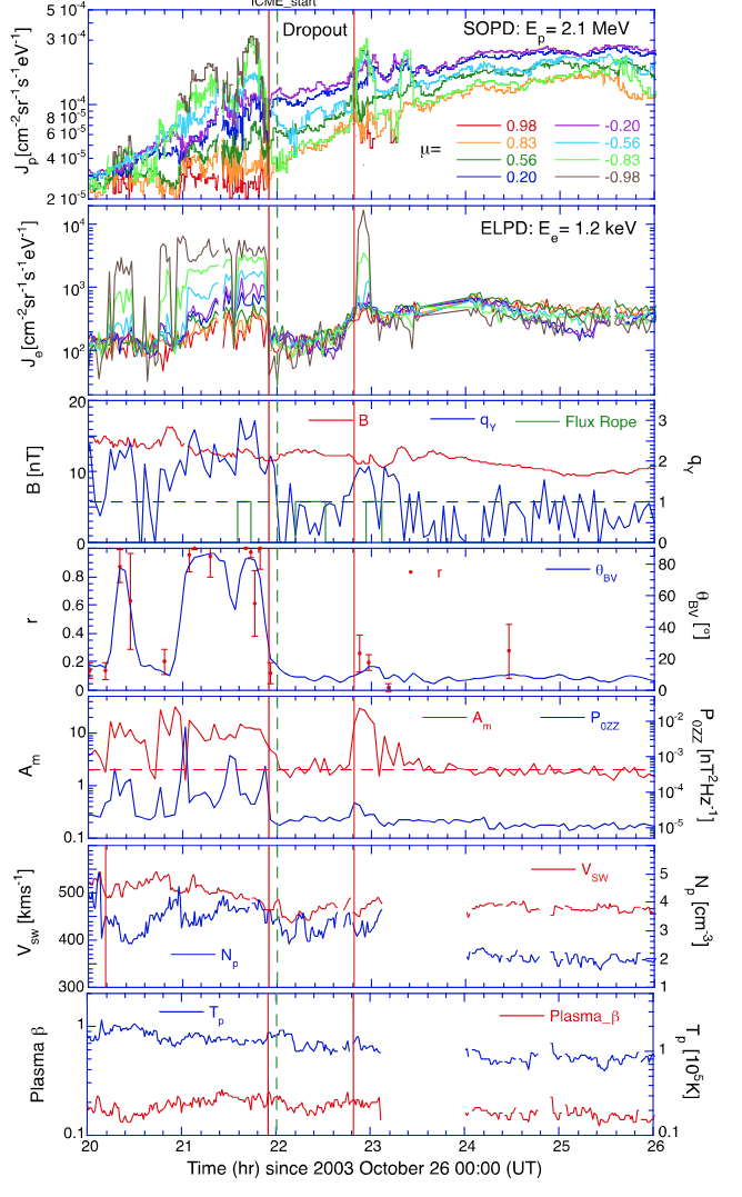
Dropouts
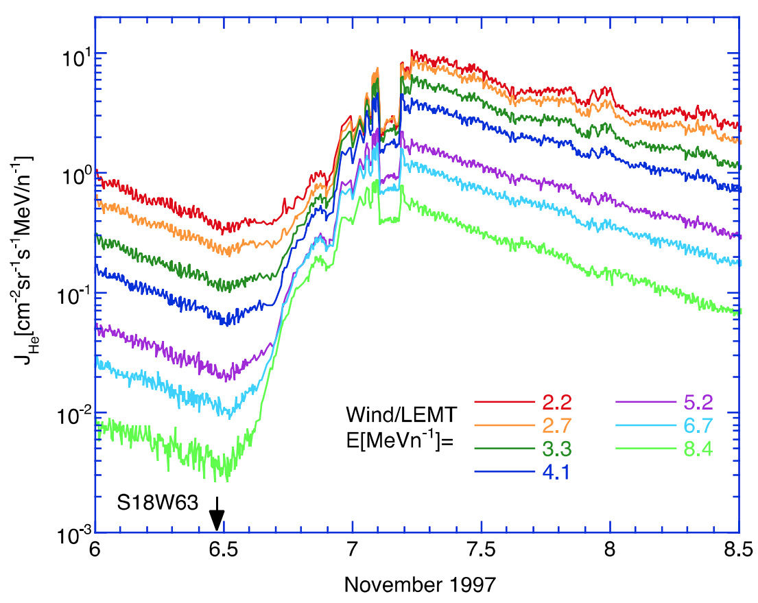
Reservoir
A region where the intensities and energy spectra throughout much of the inner heliosphere (see Fig. 52: top right panel) at different azimuthal, radial, and latitudinal locations are nearly identical
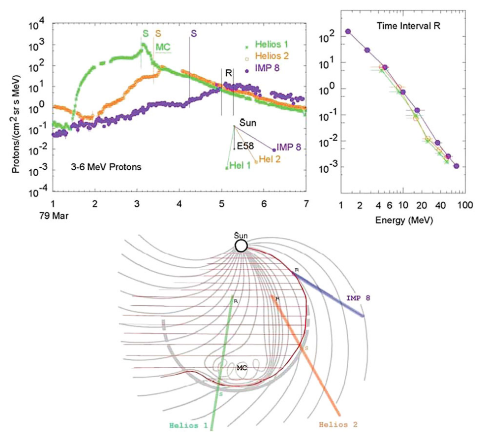
Effective cross-field and non-diffusive transport (Lario 2010)
Anomalous transport and non-Markovian phenomena
\[ \left\langle\Delta x^2(t)\right\rangle \propto t^α \]
Perri and Zimbardo (2007)
Turbulent Magnetic Fluctuations
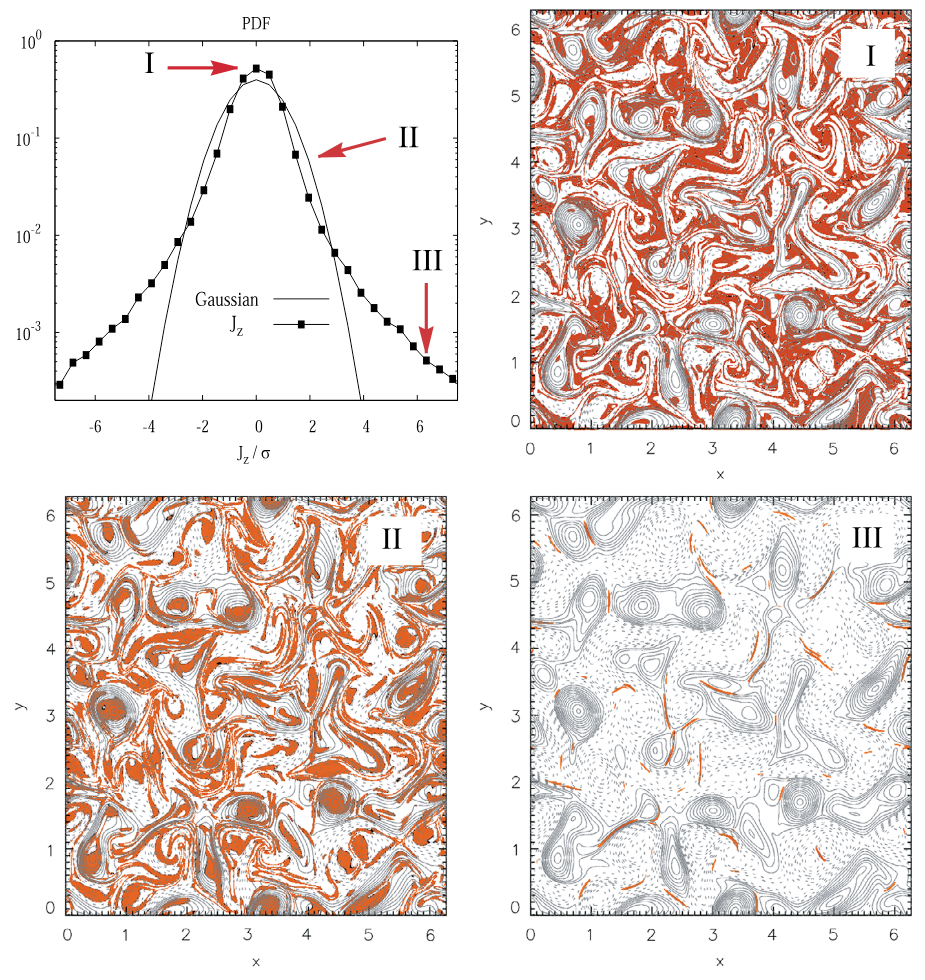
A physically appealing interpretation emerges: region I consists of very low values of fluctuations that lie mainly in the lanes between magnetic islands. Region II consists of sub-Gaussian current cores that populate the central regions of the magnetic islands (or flux tubes). Region III is composed of the coherent small-scale current sheet-like structures that form the sharp boundaries between the magnetic flux tubes. This classification provides a real-space picture of the nature of intermittent MHD turbulence.
Current sheets, rotational discontinuities (RDs), tangential discontinuities (TDs), magnetic holes,
Turbulence Transport Models (TTMs)
Broadband, low-amplitude, random-phase magnetic fluctuations
\[ \begin{aligned} & δ𝐁^s=\sum_{n=1}^{N_m} A_n\left[\cos α_n\left(\cos \phi_n \hat{x}+\sin \phi_n \hat{y}\right)+i \sin α_n(-\sin \phi_n \hat{x}+\cos \phi_n \hat{y})\right] \times \exp \left(i k_n z+i β_n\right) \\ & δ𝐁^{2 D}=\sum_{n=1}^{N_m} A_n i\left(-\sin \phi_n \hat{x}+\cos \phi_n \hat{y}\right) \times \exp \left[i k_n\left(\cos \phi_n x+\sin \phi_n y\right)+i β_n\right] \end{aligned} \tag{2}\]
Wavelet-based synthetic turbulence model (Juneja et al. 1994) similar to p-model (Meneveau and Sreenivasan 1987).
Pucci et al. (2016) studied the influence of spectral extension and intermittency on particle transport.
The Role of Current Sheets in Particle Transport
Main Scientific Objective
Motivation / Gap : No prior studies systematically characterize particle interactions with solar wind current sheets
Quantitative understanding of how these structures influence energetic particles transport
This objective leads to two main tasks:
- Observational characterization of solar wind current sheets across the heliosphere
- Development of data-driven theoretical models for current sheet-induced particle scattering and transport
Part 1: Observational Analysis of Current Sheets
“ Wanderer, there is no path the path is forged as you wander. ” - Antonio Machado
What are the properties of current sheets that are most relevant to particle transport?
Similar to the role of turbulence level, spectral index, anisotropy and intermittency in turbulence transport models
As a first-order model, we use a simple magnetic field configuration:
\[ \begin{aligned} \mathbf{B} &= B_0 (\cos θ \ \mathbf{e_z} + \sin θ ( \sin φ(z) \ \mathbf{e_x} + \cos φ (z) \ \mathbf{e_y})) \\ φ(z) &= β \tanh(z/L) \end{aligned} \]

Hamiltonian formalism
The motion of particle after simplification and normalization:
\[ \begin{aligned} \tilde{H} &= \frac{1}{2} \left(\left(\tilde{p_x}-f_1(z)\right)^2+\left(\tilde{x} \cot θ + f_2(z)\right)^2+\tilde{p_z}^2\right) \\ f_1(z) &=\frac{1}{2} \cos β \ \left(\text{Ci}\left(βs_+(z) \right)-\text{Ci}\left(βs_-(z)\right)\right) + \frac{1}{2} \sin β \ \left(\text{Si}\left(βs_+(z) \right)-\text{Si}\left(βs_-(z)\right)\right), \\ f_2(z) &=\frac{1}{2} \sin β \ \left(\text{Ci}\left(β s_+(z) \right)+\text{Ci}\left(β s_-(z)\right)\right) -\frac{1}{2} \cos β \ \left(\text{Si}\left(β s_+(z) \right)+\text{Si}\left(β s_-(z)\right)\right) \end{aligned} \tag{3}\]
Four key parameters:
- Occurrence rate
- Shear angle \(\beta\) => \(J_m = - \frac{1}{\mu_0 V_n} \frac{d B_l}{d t}\) Current density
- Normal direction \(θ\)
- Current sheet thickness (compared to the particle gyroradius)
What do we know about these parameters across the heliosphere?
Past studies Vasko et al. (2024) often lacked simultaneous multi-point measurements, employed different identification and quantification methods, and did not sufficiently separate temporal variability from spatial trends—contributing to significant uncertainties.
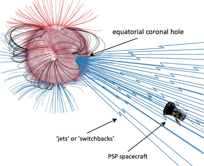
From inner heliosphere (Parker Solar Probe, PSP) to 1 AU (ARTEMIS, Wind) to outer heliosphere (Juno).
Dataset and Methods

Discontinuity Properties
Occurrence rate
Current density and thickness
Critical empirical constraints for particle transport modeling
Results and Implications
- solar wind current sheets maintain kinetic-scale thicknesses throughout the inner heliosphere
- normalized thickness and current density remain nearly constant over the range from 0.1 to 5 AU
- occurrence rates decreases approximately as \(1/r\) with radial distance between 1 and 5 AU (geometric effect)
Summary
This work is presented in “Solar wind discontinuities in the outer heliosphere: Spatial distribution between 1 and 5 AU” (Zhang et al., submitted to JGR Space Physics, 2025, manuscript is available at 10.22541/essoar.174431869.93012071/v1).
Part 2: Quantitative Modeling of Particle Scattering
In physics, you don’t have to go around making trouble for yourself – nature does it for you. - Frank Wilczek
Question: What is the specific role of coherent structures—particularly current sheets—in shaping scattering processes (as a function of particle energy and current sheet geometry)?
Approach: Combined statistical measurements of current sheets at 1 AU with a Hamiltonian analytical framework and test particle simulations.
\[ \tilde{H} = \frac{1}{2} \left(\left(\tilde{p_x}-f_1(z)\right)^2+\left(\tilde{x} \cot θ + f_2(z)\right)^2+\tilde{p_z}^2\right) \]
Adiabatic invariant and its violation at separatrix crossings
- Phase portraits of the Hamiltonian in the plane of \((z,p_z)\) at fixed \((κx, p_x)\) for \(β = 1\). Each curve corresponds to a specific \(H\), indicated on the plots. The left panel corresponds to \(\kappa x = 4\), \(p_x = 1\), while the right panel corresponds to \(\kappa x = 0\), \(p_x = 0.5\). (b) Phase plane of the Hamiltonian in the \((κx,p_x)\) space. The red line represents the uncertainty curve and the blue line delineates the boundary encompassing all possible phase points. (c) Potential energy profiles defined by \(U (z) = H − p_z^2 /2\) at different locations in the \((κx, p_x)\) place, corresponding to the labeled positions (#) in panel (b).
Part 1.5: Multifluid Model for Current Sheet Alfvénicity
The goal of physics is to find the simplest possible description that accounts for all observations.
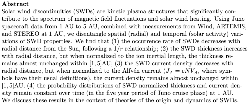
Question: Why do current sheets appear increasingly non-Alfvénic with distance, despite their force-free magnetic structure?
\[ \left(\sum_α Γ_α m_α\right) Δ v_{A,x} = \sqrt{\sum_α m_α n_α(∞) \sum_α\frac{m_α Γ_α^2 }{n_α(∞)}} ΔU_x \tag{4}\]
where \(Γ_α = n_α u_{αz}\) is constant parameter from the conservation of fluid mass.
- For a single-fluid plasma, this expression reduces to the simpler \(\Delta v_{A,x}=\Delta U_x\) f
- For two counter-streaming ion fluids with \(m_1 = m_2, u_{z,1}(∞) = -u_{z,2}(∞)\), the above expression can be further simplified to:
\[ |n_1(∞) - n_2(∞)| Δ v_{A,x} = (n_1(∞) + n_2(∞)) ΔU_x \]


Part 0: Software Development
Programming is not about typing, it’s about thinking. - Rich Hickey
PlasmaFormulary.jl: Calculation done performantly, flexibly and right. <=> plasmapy.formulary
julia> gyrofrequency(0.01u"T", :e) ≈ gyrofrequency("electron", 1e7u"nT")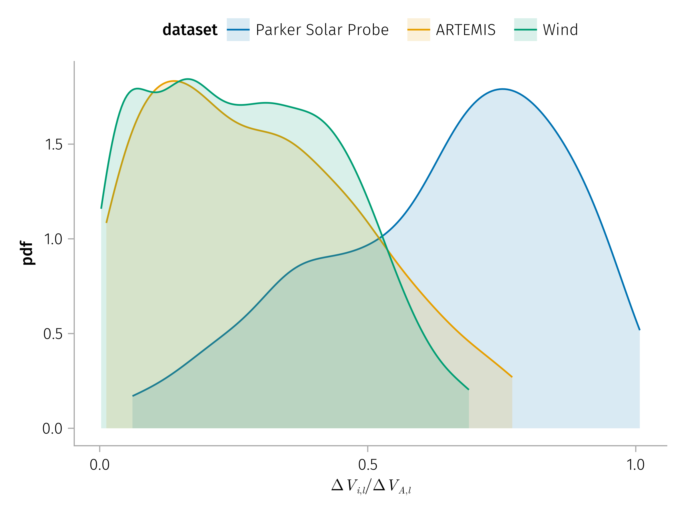
1.7588200107721632e9 rad s⁻¹ChargedParticles.jl: representing charged particles with type (memory-efficient, ready to use in test particle / PIC simulations).
julia> p = particle("Fe")
julia> p.element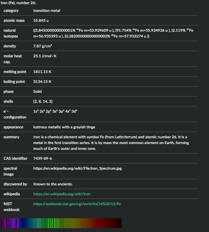
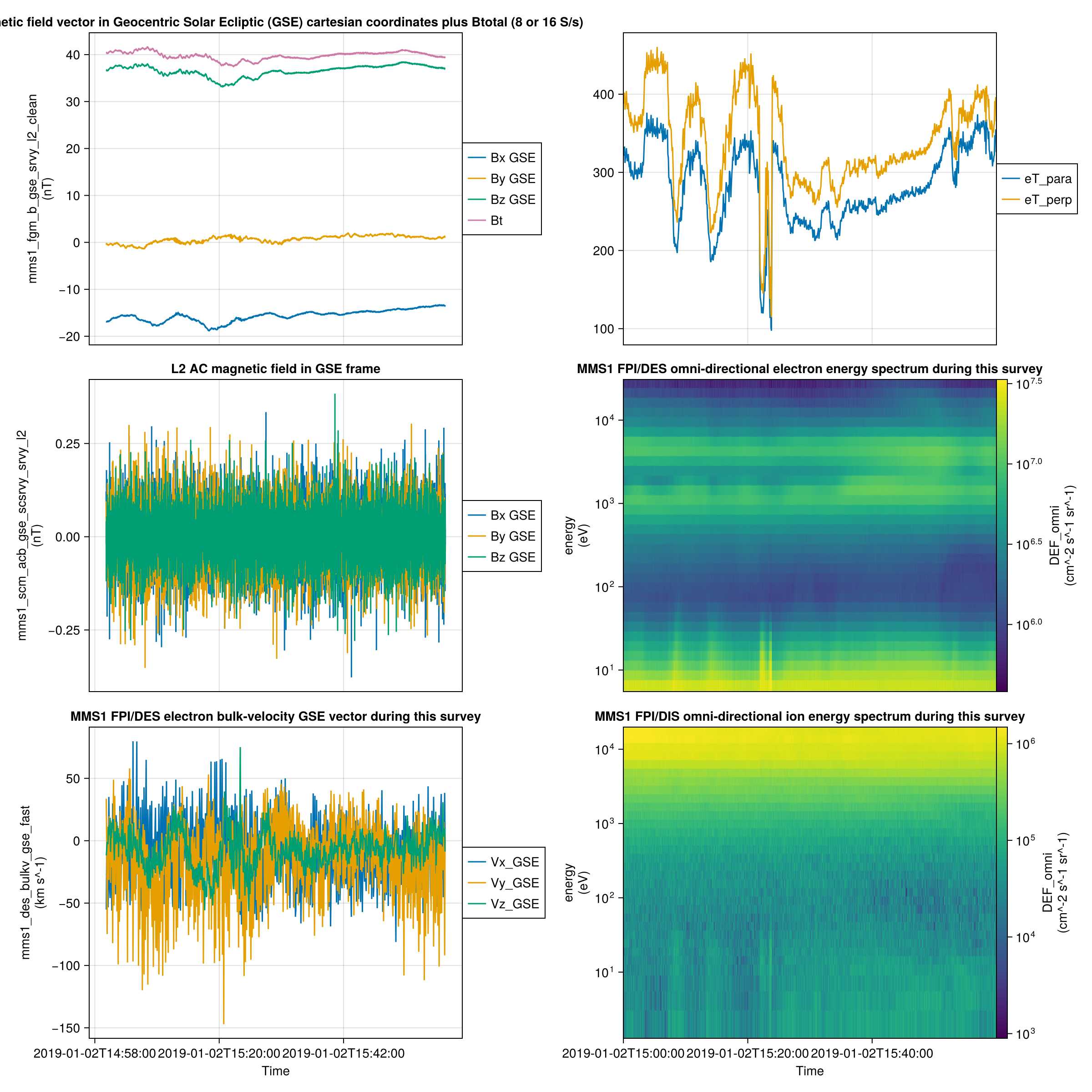
SpaceDataModel.jl: Data model for handling space/heliospheric science data: plain configuration and hierarchical abstractions. <=> SPASE metadata model.
name = "Magnetospheric Multiscale"

[metadata]
abbreviation = "MMS"

# Instruments
[instruments.fpi]
name = "Fast Plasma Investigation"
datasets = ["fpi_moms"]

[datasets.fpi_moms]
format = "MMS{probe}_FPI_{data_rate}_L2_{data_type}-MOMS"
...
[datasets.fpi_moms.metadata]
probes = [1, 2, 3, 4]
data_rates = ["fast", "brst"]
data_types = ["des", "dis"]
[datasets.fpi_moms.parameters]
numberdensity = "mms{probe}_{data_type}_numberdensity_{data_rate}"
bulkv_gse = "mms{probe}_{data_type}_bulkv_gse_{data_rate}"
temppara = "mms{probe}_{data_type}_temppara_{data_rate}"
tempperp = "mms{probe}_{data_type}_tempperp_{data_rate}"
energyspectr_omni = "mms{probe}_{data_type}_energyspectr_omni_{data_rate}"Speasy.jl: get data from main Space Physics WebServices.
PySPEDAS.jl: A Julia wrapper around PySPEDAS.
HAPIClient.jl: A Julia client for the Heliophysics Application Programmer’s Interface (HAPI).
using SPEDAS, HAPIClient, Speasy
tplot("CDAWeb/AC_H0_MFI/Magnitude,BGSEc", "2001-1-2", "2001-1-2T12")
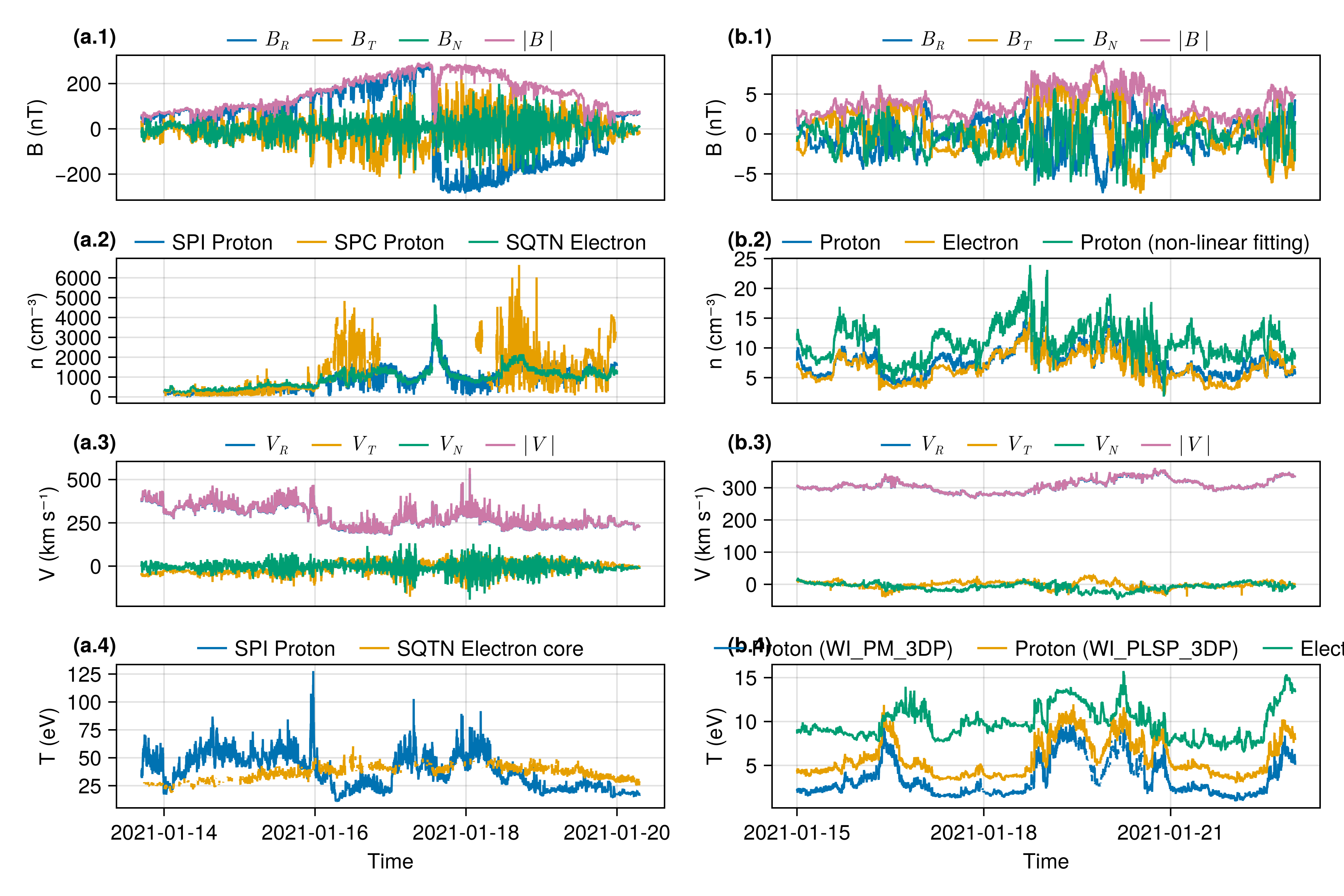
n = DataSet("Density",
[
SpeasyProduct("PSP_SWP_SPI_SF00_L3_MOM/DENS"; labels=["SPI Proton"]),
Base.Fix2(*, u"cm^-3") ∘ SpeasyProduct("PSP_SWP_SPC_L3I/np_moment"; labels=["SPC Proton"]),
SpeasyProduct("PSP_FLD_L3_RFS_LFR_QTN/N_elec"; labels=["RFS Electron"]),
SpeasyProduct("PSP_FLD_L3_SQTN_RFS_V1V2/electron_density"; labels=["SQTN Electron"])
]
)
tplot(n, "2021-08-09T06", "2021-08-10T18")
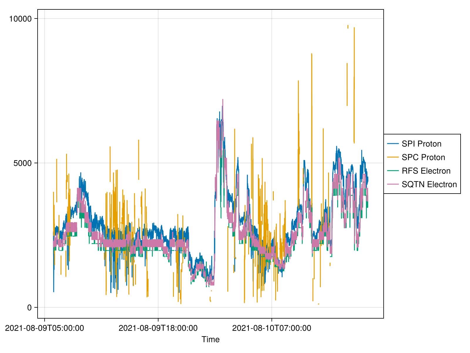
Speasy.jlSPEDAS.jl : Julia-based Space Physics Environment Data Analysis Software framework.
SPEDAS.jl: Plotting multiple time series on a single figurePart 3: Proposed Research
“ But still try, for who knows what is possible? ” - Michael Faraday
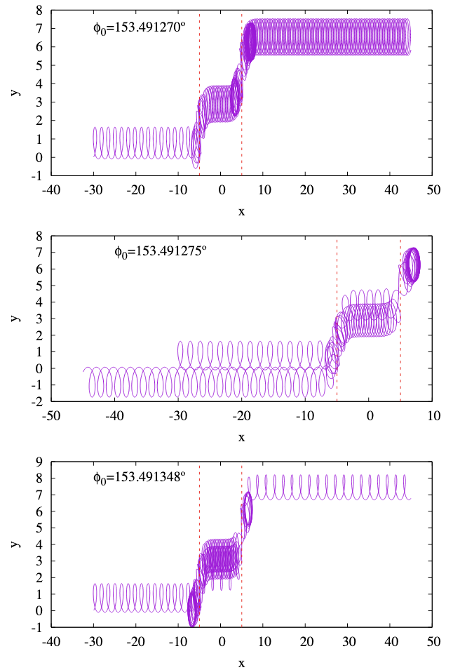
The total time between two consecutive current sheet encounters is modeled as the sum of the time spent inside the current sheet \(T_{cs}\), and the time spent free-streaming between sheets \(T_{fs}\), given by:
\[ T = T_{cs} + T_{fs}, \quad T_{fs} = \frac{s_{fs}}{|v_{∥,1}|} \]
where \(v_{∥,0}\), \(v_{∥,1}\) are the particle’s changed parallel velocity before and after interacting with the current sheet, respectively.
In the absence of scattering, the particle would follow the field line and travel a distance:
\[ s_0 = |v_{∥,0}| \cdot T = |v_{∥,0}| \left( T_{cs} + \frac{s_{fs}}{|v_{∥,1}|} \right). \]
However, when scattering occurs, the total distance traveled becomes:
\[ s = s_{cs}^* + \text{sign}\left(\frac{v_{∥,1}}{v_{∥,0}}\right) s_{fs} \approx \text{sign}\left(\frac{v_{∥,1}}{v_{∥,0}}\right) s_{fs} \]
under the approximation that \(s_{cs}^* << s_{fs}\), where \(s_{cs}^*\) is the effective parallel distance the particle travels within the current sheet. The net displacement compared to the unperturbed case is then:
\[ Δ s_∥ = s - s_0 = s_{fs} \left(\text{sign}\left(\frac{v_{∥,1}}{v_{∥,0}}\right) - \frac{|v_{∥,0}|}{|v_{∥,1}|} \right) - |v_{∥,0}| T_{cs} \]
The parallel spatial diffusion coefficient is then expressed as:
\[ κ_∥ = \frac{(Δ s_∥)^2}{Δ t} \]
Similarly, for the perpendicular direction:
\[ κ_\perp = \frac{(Δ s_\perp)^2}{T_{cs} + | s_{fs} / v_{∥,1} |}. \]
Conclusion
“ Still round the corner there may wait A new road or a secret gate ” - J. R. R. Tolkien
Timeline
Months 1–4:
Refine the pitch-angle scattering model to incorporate both parallel and perpendicular spatial diffusion effects.
Conduct detailed test-particle simulations using solar wind parameters derived from multi-spacecraft observations (PSP, Wind, Juno, etc.).
Months 5–7:
Identify observational signatures supporting the proposed scattering model.
Examine how current sheet properties influence SEP scattering across different heliocentric distances.
Months 8–10:
Finalize the spatial diffusion model and assess its implications for large-scale SEP propagation.
Synthesize simulation results and observational insights into dissertation chapters. Integrate observational and theoretical findings into comprehensive thesis documentation.
Opportunities for Future Research
Completion of this thesis opens several avenues for future investigations:
Exploration of current sheet interactions in other astrophysical environments, such as planetary magnetospheres.
Advanced integration of mapping techniques with numerical simulations to further refine SEP transport models.
Expanded observational campaigns utilizing upcoming spacecraft missions designed to probe heliospheric turbulence and particle dynamics at unprecedented resolution.